K-Means Clustering
Contents
17.4. K-Means Clustering#
An initial version of the k-means algorithm was originally developed by Lloyd in 1957 but was published for the first time in 1982 [57].
Given a set of \(n\) data points in \(\RR^m\), the objective is to select \(k\) centroids so as to minimize the sum of squared distances between each point and its closest centroid. In general the problem is NP-hard but a local search method to this problem as described in Algorithm 17.1 is generally quite successful in finding reasonable solutions.
See [29, 46, 59] for a detailed treatment of the algorithm.
17.4.1. Basic Algorithm#
K-means clustering algorithm is a hard clustering algorithm as it assigns each data point to exactly one cluster.
Algorithm 17.1 (Basic k-means clustering algorithm)
Select \(k\) points as initial centroids.
Repeat
Segmentation: Form \(k\) clusters by assigning all points to the nearest centroid.
Estimation: Recompute the centroid for each cluster.
Until the segmentation has stopped improving.
The input to an algorithm is an unlabeled dataset
\[ \bX = \{ \bx_1, \bx_2, \dots, \bx_n \} \]where each data point belongs to the ambient feature space \(\RR^m\).
Our goal is to partition the dataset into \(k\) different clusters.
The clustering is denoted by
\[ \CCC = \{C_1, \dots, C_k \} \]where \(C_j\) is the list of indices of data points belonging to the \(j\)-th cluster.
The clustering can be conveniently represented in the form of a label array \(L\) consisting of \(n\) entries each of which can take a value from \(\{ 1, \dots, k \}\).
In other words, if \(L[i] = j\), then the data point \(\bx_i\) belongs to the \(j\)-th cluster (\(i \in C_j\)).
Each cluster \(C_j\) is represented by a centroid (or a mean vector) \(\mu_j\).
The algorithm consists of two major steps:
Segmentation
Estimation
The goal of segmentation step is to partition the data points into clusters according to the nearest cluster centroids.
The goal of estimation step is to compute the new centroid for each cluster based on the current clustering.
\[ \mu_j = \frac{1}{n} \sum_{i \in C_j} \bx_i. \]We start with an initial set of centroids for each cluster.
One way to pick the initial centroids is to pick \(k\) points randomly from the dataset.
In each iteration, we segment the data points into individual clusters by assigning a data point to the cluster corresponding to the nearest centroid.
Then, we estimate the new centroid for each cluster.
We return a labels array \(L\) which maps each point to corresponding cluster.
We note that the basic structure of the k-means is not really an algorithm. It is more like a template of the algorithm. For a concrete implementation of the k-means algorithm, there are many aspects that need to be carefully selected.
Initialization of the centroids
Number of clusters
Choice of the distance metric
Criterion for evaluation of the quality of the clustering
Stopping criterion
17.4.1.1. Example#
Example 17.7 (A k-means example)
We show a simple simulation of k-means algorithm.
The data consists of randomly generated points organized in 4 clusters.
The algorithm is seeded with random points at the beginning.
After each iteration, the centroids are moved to a new location based on the current members of the cluster.
The animation below shows how the centroids are moving and cluster memberships are changing.
Fig. 17.6 This animation shows how the centroids move from one iteration to the next. The centroids have been initialized randomly in the first iteration.#
The figure below shows the clusters and centroids of all the six iterations in a grid. You can open this figure in a different tab to see its enlarged version.
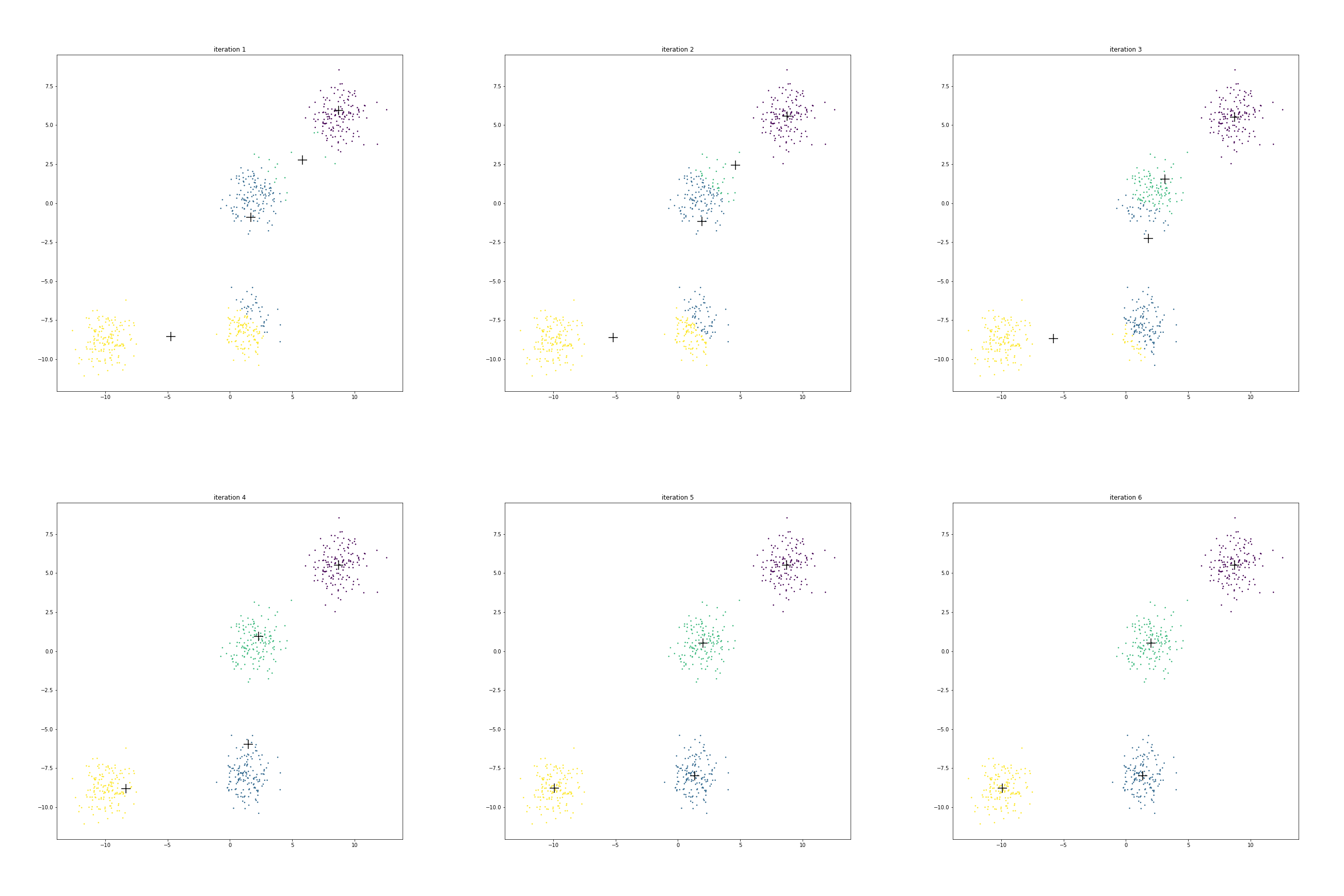
We have 4 centroids randomly initialized at iteration 1. Let us call them as
A near \((-5, -8)\) (centroid of yellow cluster)
B near \((1.5, -1)\) (centroid of blue cluster)
C near \((6, 2.5)\) (centroid of the green cluster)
D near \((8.5, 6)\) (centroid of the purple cluster)
Look at centroid A over time
It starts from the location \((-5, -8)\).
More than half of the points from the eventual blue cluster are still belonging to the yellow cluster in the first iteration.
As the centroid starts moving towards its eventual location near \((-9, -8.5)\), extra points from the yellow cluster are dropped.
Next look at the journey of centroid B.
In the beginning it contains about 70% points of the cluster around origin and only about 20% points of the cluster around \((1.5, -7.5)\).
But it is enough to start pulling the centroid downward.
As the centroid C starts moving left & down, the points around origin start becoming green.
Since centroid A is also moving left, the points around \((1.5, -7.5)\) start turning blue.
Centroid D doesn’t really move much.
Initially it is in competition with centroid C for some of its points around its boundary.
However as C starts moving to its final destination, all the points around D turn purple.
Since not many points had to change cluster membership here, hence their centroid location didn’t shift much over these iterations.
We also note that after iteration 5, there is no further change in cluster memberships. Hence the centroids stop moving.
17.4.1.2. Stopping Criterion#
As we noticed that in the previous example that centroids converge fast during the initial iterations and then they start moving very slowly. Once the segmentation stops changing, then the centroids will also stop moving. When the cluster boundaries are not clear, it is often good enough to stop the algorithm when relatively very few points are changing clusters.
17.4.1.3. Evaluation#
A simple measure for the evaluation of the k-means algorithm is the within-cluster-scatter given by
As can be seen from the formula, this is essentially the sum of squared errors w.r.t. the corresponding cluster centroids.
17.4.1.4. Convergence#
It can be shown that the scatter is monotonically decreasing over the k-means iterations.
One can easily see that there are only at most \(k^n\) possible clusterings.
Each partition has a different value of scatter.
Since the scatter is monotonically decreasing, hence no configuration is repeated twice.
Since the number of possible clusterings is finite, hence the algorithm must terminate eventually.
17.4.1.5. Number of Clusters#
The algorithm requires that the user provide the desired number of clusters \(k\) as an input to the algorithm. It doesn’t discover the the number of clusters automatically. We can also see that one straight-forward way to decrease the within cluster scatter is to increase the number of clusters. In fact, when \(k=n\), then the optimal within cluster scanner will be \(0\). However, a lower scatter may provide a clustering which will not be very useful.
This begs the question how do we select the number of clusters? Here are a few choices:
Run the algorithm on the data with different values of \(k\) and then choose a clustering by inspecting the results.
Use another clustering method like EM.
Use some domain specific prior knowledge to decide the number of clusters.
17.4.1.6. Initialization#
There are a few options for selection of initial centroids:
Randomly chosen data points from the data set.
Random points in the feature space \(\RR^m\).
Create a random partition of \(\bX\) into \(k\) clusters and take the centroid of each partition.
Identify regions of space which are dense (in terms of number of data points per unit volume) and then select points from those regions as centroids.
Uniformly spaced points in the feature space.
Later, we will discuss a specific algorithm called k-means++ which carefully selects the initial centroids.
k-means algorithm doesn’t provide a globally optimal clustering for a given number of clusters. It does converge to a locally optimal solution based on the initial selection of the centroids.
One way to address this is to run the k-means algorithm multiple times with different initializations. At the end, we select the clustering with the smallest scatter.
17.4.2. Scale and Correlation#
One way to address the issue of scale variation in features and correlation among features is using the Mahalanobis distance for distance calculations. To do this, in the estimation step we shall calculate the covariance matrix for each cluster separately.
Algorithm 17.2 (k-means clustering with Mahalanobis distance)
Inputs:
The data set \(\bX = \{ \bx_s\}_{s=1}^n \subset \RR^m\)
Number of clusters : \(k\)
Outputs:
Clusters: \(\{\bX_j^{(i)} \}_{j=1}^k\)
Cluster labels array: \(L[1:n]\)
Initialization:
\(i \leftarrow 0\). # Iteration counter
For each cluster \(j \in \{1, \dots, k\}\):
Initialize \(\mu_j^{(0)}\) and \(\Sigma_j^{(0)}\) suitably.
Set \(\bX_j^{(0)}\) to empty set.
Algorithm:
If the segmentation has stopped changing: break.
Segmentation: for each data point \(\bx_s \in \bX\):
Find the nearest centroid via Mahalanobis distance.
\[ L(s) \leftarrow l \leftarrow \underset{j=1,\dots, k}{\text{arg min}} \| \bx_s - \mu_j^{(i)} \|^2_{\Sigma_j^{(i)}}. \]Use the centroid number as the label for the point.
Assign \(\bx_s\) to the cluster \(\bX_l^{(i+1)}\).
Estimation: for each cluster \(j \in \{1, \dots, k\}\):
Compute new mean/centroid for the cluster:
\[ \mu_j^{(i+1)} \leftarrow \text{mean}(\bX_j^{(i+1)}). \]Compute the covariance matrix for the cluster:
\[ \Sigma_j^{(i+1)} \leftarrow \text{cov}(\bX_j^{(i+1)}). \]
\(i \leftarrow i+1\). # Increase iteration counter
Go to step 1.
A within-cluster-scatter can be defined as
This represents the average (squared) distance of each point to the respective cluster mean. The \(k\)-means algorithm reduces the scatter in each iteration. it is guaranteed to converge to a local minimum.