Introduction
Contents
17.1. Introduction#
The objective of data clustering is to group objects so that objects in the same group are similar to each other while objects in different groups are quite distinct from each other. Each group is known as a cluster.
Data clustering is different from classification. In a data classification problem, objects are assigned to one of the predefined classes. In a clustering problem, the classes are not known in advance. We discover the classes as a result of the data clustering process itself.
17.1.1. Examples#
Example 17.1 (Market research)
Clustering is often used in market research. One particular application is market segmentation.
Data is collected about which customer is buying which product
Basic demographic information (age, location, gender) is collected for each customer.
Clustering is used to identify groups of customers with similar needs and budgets.
Based on this market segmentation information, targeted marketing campaigns can be executed to promote matching products to individual segments.
Example 17.2 (Image segmentation)
A digital image is a collection of pixels (with RGB components). However, a viewer doesn’t see those individual pixels but sees real objects depicted by those pixels (trees, buildings, faces, people, cars, machines, animals, etc.). The objective of image segmentation is to split the image into groups of pixels which represent individual objects being perceived by humans. Data clustering techniques are often used to detect borders between the objects in an image.
Example 17.3 (Professional basketball)
In professional basketball, one common problem is to identify players who are similar to each other. One can collect a number of player statistics
points per game
rebounds per game
assists per game
steals per game
Once this data for individual players has been obtained, one can run a clustering algorithm to identify groups of players who are similar to each other in playing styles. This data is valuable in planning for practice, drills, player selection etc..
Example 17.4 (Health insurance)
In health insurance, one major activity is to come up with suitable insurance packages based on the varying needs of different households.
One may collect following data for each household
Household size
Number of doctor visits per year
Number of chronic conditions
Number of children
Number of adults
Average age
One may cluster this data to identify households that are similar. Suitable insurance packages with corresponding monthly premiums can be designed to target these clusters of households.
From these examples we can see that in different clustering problems, different types of objects/things are being clustered.
Pixels in an image
Player statistics
Customer demographics and purchase data
Household demographics and clinical data
In order to mathematically analyze the data, it is important to map the data into some high dimensional Euclidean space \(\RR^m\). Then individual objects/things get represented as data points in the Euclidean space. The clustering problem then reduces to group points which are similar to each other.
A key question is how to measure similarity between different data points.
17.1.2. Vocabulary#
We provide an informal definition of a dataset on which clustering is applied.
17.1.2.1. Dataset#
Definition 17.1 (Dataset)
A dataset consists of one or more records. A record is also known as a data point, observation, object, item, or tuple. A record is represented as a point in a high dimensional Euclidean space. Thus, a dataset is a collection of points in the Euclidean space.
The individual scalar components of a data point are known as variable, attribute or feature.
The number of features or variables is the dimension of the Euclidean space from which the dataset has been drawn.
Mathematically, the dataset is a collection of \(n\) data points (or objects), each of which is described by \(m\) attributes, denoted by \(\bX\) as
where each
for \(i=1,\dots,n\) is a vector denoting the \(i\)-th object. \(x_{i j}\) is the \(j\)-th scalar component (attribute) of the \(i\)-th object. The dimensionality of the dataset is the number of attributes \(m\).
We shall often abuse the notation and say that \(\bX\) also represents the \(m \times n\) data-matrix
17.1.2.2. Distance and Similarity#
The key idea in data clustering is that objects belonging to the same cluster look similar to each other and objects belonging to different clusters look distinct from each other. In order to give this idea a concrete shape, we need to introduce some means to measure the similarity between objects. Since the objects are represented using points in the Euclidean space \(\RR^m\), hence one natural way to measure similarity is to measure the distance between the points. The closer the points are to each other, the more similar they are. Once the objects have been organized into clusters, one can also wonder about ways to quantify how similar or dissimilar the clusters are with each other.
Data clustering literature consists of hundreds of different similarity measures, dissimilarity measures, and distance metrics to quantify the similarity or dissimilarity between different objects being clustered. The choice of a particular metric depends heavily on a particular application.
Distances and similarities are essentially reciprocal concepts. In distance based clustering, we group the points into \(k\) clusters such that the distance among points in the same group is significantly smaller than those between clusters.
In similarity based clustering, the points within the same cluster are more similar to each other than points from different cluster.
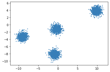
Fig. 17.1 2D Raw data (2 features) before clustering#
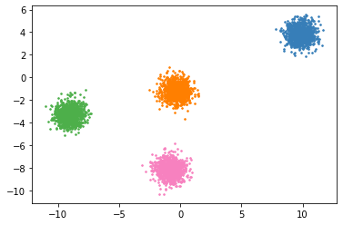
Fig. 17.2 Different clusters have been identified based on a distance metric. Nearby points fall in the same cluster (identified by same color).#
A simple way to measure similarity between two points is the absolute value of the inner product. Alternatively, one can look at the angle between two points or inner product of the normalized points. Another way to measure similarity is to consider the inverse of an appropriate distance measure.
A simple similarity or distance based measure may not be suitable by itself for performing the clustering in all cases.
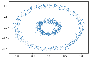
Fig. 17.3 From visual inspection it appears that the data is organized into two separate rings. However, a distance metric will not be able to segregate data into rings. The points in the inner ring are closer to the right end of the outer ring than the points in the left end of the outer ring.#
There are more sophisticated approaches available A graph based clustering algorithm treats each data point as a vertex on a graph [with appropriate edges]. Edges are typically weighted where the weight is proportional to the similarity between two points or the inverse of distance between two points. The algorithm then attempts to divide the graph into strongly connected components.
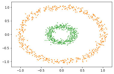
Fig. 17.4 Ideal clustering of this data should be able to segregate the two rings correctly. If we carefully see the image we can observe that while the distance between the left and right far ends of the outer ring is large, there is a series of points on the ring which are close to each other forming a chain from one end to the other. Thus, if we form a graph where edge strengths are proportional to the inverse of distance between points, then all the points in individual rings will form very strong connected components while the edges between points from the two rings will be very weak.#
17.1.2.3. Distance Metrics#
Simplest distance measure is the standard Euclidean distance measure. The Euclidean distance between two points \(\bx, \by \in \bX\) is given by
Euclidean distance is susceptible to the choice of basis.
Example 17.5 (Susceptibility of Euclidean metric)
Consider a dataset which consists of two features of individuals
age
height
When we collect the data the unit of measurement becomes important.
If age is measured in seconds and height in meters then the Euclidean distance will be dominated by difference in age. The difference in height will get largely ignored.
If age is measured in years and height is measured in millimeters, then the Euclidean distance will be dominated by the difference in height.
If age is measured in decades and height in feet, then both features will have similar ranges.
There is still the issue of correlation between age and height. As age increases, height also increases.
The correlation in age and height is superfluous information and is not really useful in the clustering objective.
This can be improved by adopting a statistical model for data in each cluster. We assume that the data in \(k\)-th cluster is sampled from a probability distribution with mean \(\mu_k\) and covariance \(\Sigma_k\). An appropriate distance measure from the mean of a distribution which is invariant of the choice of basis is the Mahalanobis distance:
For Gaussian distributions, this is proportional to the negative of the log-likelihood of a sample point.
17.1.2.4. Clusters#
The data clustering process divides the objects belonging to the dataset into clusters or groups or classes. These terms are used interchangeably in the literature. There is no formal definition of what a cluster means however we can provide some basic criteria which objects within a cluster will generally meet:
The objects will share the same or closely related properties.
The data points will show small mutual distances or dissimilarities (at least to a few points within the same cluster)
The objects will have contacts or relations with at least one object within the cluster
The objects within a cluster will be clearly distinguishable from the objects in the rest of the dataset.
In the 2-D/3-D visualizations of the data points, we can often see empty space between different clusters if the data is amenable to clustering.
Definition 17.2 (Compact cluster)
A compact cluster is a set of data points in which the members have high mutual similarity.
The clusters in Fig. 17.2 are examples of compact clusters.
Usually a compact cluster can be represented by an representative point or a centroid of points within the cluster. In categorical data, a mode of the points within a cluster may be more appropriate.
Definition 17.3 (Chained cluster)
A chained cluster is a set of data points in which every member is more similar to some members within the cluster than other data points outside the cluster.
The two rings in Fig. 17.4 are very good examples of chained clusters.
17.1.2.5. Hard vs Soft Clustering#
So far we have discussed clustering in a way where each object in the dataset is assigned to exactly one cluster. This approach is called hard clustering.
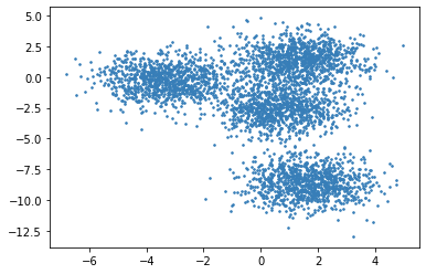
Fig. 17.5 Careful visual inspection suggests that the data seems to have 4 different clusters. However, there are no clear boundaries between different clusters as there is not enough empty space around them. It is very difficult to decide how to place the data in the boundary regions into different clusters.#
A more nuanced approach is to allow for fuzzy or probabilistic membership to different clusters.
We postulate that the dataset consists of \(k\) cluster.
We say that the \(i\)-th data point belongs to the \(j\)-th cluster with a probability \(u_{i j}\).
We require that \(u_{i j} \geq 0\) for every \(i\) and \(j\).
We require that
\[ \sum_{j=1}^k u_{i j} = 1. \]In other words, \(\{u_{i 1}, \dots, u_{i k} \}\) form a probability distribution of membership of the \(i\)-th object to different clusters.
We also require that
\[ \sum_{i=1}^n u_{i j} > 0. \]In other words, every cluster has at least some soft membership from some data points.
This type of clustering assignment is known as soft clustering.
We can put together all the membership values \(u_{i j}\) into an \(n \times k\) matrix
We can see that hard clustering is a special case of soft clustering where we require that \(u_{i j} \in \{ 0, 1 \}\) for every \(i\) and every \(j\).
The matrix \(\bU\) is often known as a \(k\)-partition. In hard clutering, it is known as a hard \(k\)-partition. In soft clustering, it is known as a fuzzy \(k\)-partition.
Definition 17.4 (\(k\) partition)
Let \(\bX\) be a dataset of \(n\) points. Assume that \(\bX\) is clustered into \(k\) clusters given by an \(n \times k\) matrix \(\bU\). Then the matrix \(\bU\) is called a \(k\)-partition of the dataset \(\bX\).
If it is a hard clustering where each object belongs to exactly one cluster, then \(\bU\) is called a hard \(k\)-partition. If a soft clustering has been applied such that every data item can belong to different clusters in a probabilistic manner, then the matrix \(\bU\) is called a fuzzy \(k\) partition of \(\bX\).
Soft clustering relaxes the constraint that every object belongs to exactly one cluster and allows the flexibility of partial memberships into different clusters.
Looking back at Fig. 17.5, we can see that a soft clustering approach may be more sensible for this kind of dataset where the boundaries between clusters are not clear. It also clarifies that while for many points near the centers of the clusters we can be fairly certain about which clusters they belong to, it is the points around the boundaries between the clusters which benefit a lot from the soft assignments.
17.1.3. Clustering Algorithms#
There are two general classes of clustering algorithms
Hierarchical algorithms
Partitioning algorithms
17.1.3.1. Hierarchical Algorithms#
There are two types of hierarchical algorithms.
Divisive algorithms
Agglomerative algorithms
In a divisive algorithm, one proceeds from top to bottom, starting with one large cluster containing the entire data set and then splitting the clusters recursively till there there is no further need to split more.
In an agglomerative algorithm, one starts with one cluster per data point and then keeps merging clusters till the time further merging of clusters doesn’t make sense.
Hierarchical algorithms typically consume \(\bigO(n^2)\) memory and \(\bigO(n^3)\) CPU time where \(n\) is the number of data points. Hence, they tend to become impractical for large datasets unless special techniques are employed to mitigate the excessive resource requirements.
17.1.3.2. Partitioning Algorithms#
Unlike hierarchical algorithms, the partitioning algorithms directly split the data into a suitable number of clusters.
Some of the popular algorithms are
\(k\)-means clustering
spectral clustering
expectation maximization