9.8. Convex Functions

Throughout this section, we assume that $\mathbb{V},\mathbb{W}$ are real vector spaces. Wherever necessary, they are equipped with a norm $\Vert \cdot \Vert$ or an real inner product $⟨\cdot ,\cdot ⟩$. They are also equipped with a metric $d(\mathbf{x},\mathbf{y})=\Vert \mathbf{x}-\mathbf{y}\Vert$ as needed.

We suggest the readers to review the notions of graph, epigraph, sublevel sets of real valued functions in Real Valued Functions. Also pay attention to the notion of extended real valued functions, their effective domains, graphs and level sets.

9.8.1. Convexity of a Function

Definition 9.43 (Convex function)

Let $\mathbb{V}$ be a real vector space. A real valued function $f:\mathbb{V}\to \mathbb{R}$ is convex if $\mathrm{dom}f$ is a convex set and for all ${\mathbf{x}}_1,{\mathbf{x}}_2\in \mathrm{dom}f$, and $t\in [0,1]$, we have:

(9.1)$$f(t{\mathbf{x}}_1+(1-t){\mathbf{x}}_2)\le tf({\mathbf{x}}_1)+(1-t)f({\mathbf{x}}_2).$$

An extended valued function $f:\mathbb{V}\to \bar{\mathbb{R}}$ is convex if $\mathrm{dom}f$ is a convex set and for every ${\mathbf{x}}_1,{\mathbf{x}}_2\in \mathbb{V}$, and $t\in [0,1]$, we have:

$$f(t{\mathbf{x}}_1+(1-t){\mathbf{x}}_2)\le tf({\mathbf{x}}_1)+(1-t)f({\mathbf{x}}_2).$$

Fig. 9.3 Graph of a convex function. The line segment between any two points on the graph lies above the graph.

For a convex function, every chord lies above the graph of the function.

9.8.1.1. Strictly Convex Functions

Definition 9.44 (Strictly convex function)

Let $\mathbb{V}$ be a real vector space. A convex function $f:\mathbb{V}\to \mathbb{R}$ is strictly convex if for all ${\mathbf{x}}_1,{\mathbf{x}}_2\in \mathrm{dom}f$, where ${\mathbf{x}}_1$ and ${\mathbf{x}}_2$ are distinct, and $t\in (0,1)$, we have:

$$f(t{\mathbf{x}}_1+(1-t){\mathbf{x}}_2)<tf({\mathbf{x}}_1)+(1-t)f({\mathbf{x}}_2).$$

In other words, the inequality is a strict inequality whenever the point $\mathbf{x}=t{\mathbf{x}}_1+(1-t){\mathbf{x}}_2$ is distinct from ${\mathbf{x}}_1$ and ${\mathbf{x}}_2$ both.

9.8.1.2. Concave Functions

Definition 9.45 (Concave function)

We say that a function $f$ is concave if $-f$ is convex. A function $f$ is strictly concave if $-f$ is strictly convex.

Example 9.25 (Linear functional)

A linear functional on $\mathbb{V}$ in an inner product space has the form of an inner product parameterized by a vector $\mathbf{a}\in \mathbb{V}$ as

$$f_{\mathbf{a}}(\mathbf{x})\triangleq ⟨\mathbf{x},\mathbf{a}⟩\mathrm{\forall }\mathbf{x}\in \mathbb{V}.$$

i.e. the inner product of $\mathbf{x}$ with $\mathbf{a}$.

Theorem 9.67

All linear functionals on a real vector space are convex as well as concave.

Proof. For any $\mathbf{x},\mathbf{y}\in \mathbb{V}$ and $t\in [0,1]$:

$$\begin{array}{rl}{f}_{\mathbf{a}}(t\mathbf{x}+(1-t)\mathbf{y})& =⟨t\mathbf{x}+(1-t)\mathbf{y},\mathbf{a}⟩\\ & =t⟨\mathbf{x},\mathbf{a}⟩+(1-t)⟨\mathbf{x},\mathbf{a}⟩\text{inner products are linear}\\ & =t{f}_{\mathbf{a}}(\mathbf{x})+(1-t)f_{\mathbf{a}}(\mathbf{y}).\end{array}$$

Thus, $f_{\mathbf{a}}$ is convex. We can also see that $-f_{\mathbf{a}}$ is convex too. Hence, $f_{\mathbf{a}}$ is concave too.

9.8.1.3. Arithmetic Mean

Example 9.26 (Arithmetic mean is convex and concave)

Let $f:{\mathbb{R}}^n\to \mathbb{R}$ be given by:

$$f(\mathbf{x})=\frac{x_1+\cdots +x_n}{n}.$$

Arithmetic mean is a linear function. In fact

$$\begin{array}{rl}f(\alpha \mathbf{x}+\beta \mathbf{y})& =\frac{1}{n}(\sum _{i=1}^n(\alpha x_i+\beta y_i))\\ & =\alpha \frac{x_1+\cdots +x_n}{n}+\beta \frac{y_1+\cdots +y_n}{n}\\ & =\alpha f(\mathbf{x})+\beta f(\mathbf{y})\end{array}$$

for all $\alpha ,\beta \in \mathbb{R}$.

Thus, for $t\in [0,1]$

$$f(t\mathbf{x}+(1-t)\mathbf{y})=tf(\mathbf{x})+(1-t)f(\mathbf{y}).$$

Thus, arithmetic mean is both convex and concave.

9.8.1.4. Affine Function

Example 9.27 (Affine functional)

An affine functional is a special type of affine function which maps a vector from $\mathbb{V}$ to a scalar in the associate field $\mathbb{F}$.

On real vector spaces, an affine functional on $\mathbb{V}$ is defined in terms of a vector $\mathbf{a}\in \mathbb{V}$ and a scalar $b\in \mathbb{R}$ as

$$f_{\mathbf{a},b}(\mathbf{x})\triangleq ⟨\mathbf{x},\mathbf{a}⟩+b\mathrm{\forall }\mathbf{x}\in \mathbb{V}$$

i.e. the inner product of $\mathbf{x}$ with $\mathbf{a}$ followed by a translation by the amount of $b$.

Theorem 9.68

All affine functionals on a real vector space are convex as well as concave.

Proof. A simple way to show this is to recall that for any affine function $T$,

$$T(t\mathbf{x}+(1-t)\mathbf{y})=tT(\mathbf{x})+(1-t)T(\mathbf{y})$$

holds true for any $\mathbf{x},\mathbf{y}\in \mathbb{V}$ and $t\in \mathbb{F}$.

In the particular case of real affine functionals, for any $\mathbf{x},\mathbf{y}\in \mathbb{V}$ and $t\in [0,1]$, the previous identity reduces to:

$$f_{\mathbf{a},b}(t\mathbf{x}+(1-t)\mathbf{y})=t{f}_{\mathbf{a},b}(\mathbf{x})+(1-t)f_{\mathbf{a},b}(\mathbf{y}).$$

This establishes that $f_{\mathbf{a},b}$ is both convex and concave.

Another way to prove this is by following the definition of $f_{\mathbf{a},b}$ above:

$$\begin{array}{rl}{f}_{\mathbf{a},b}(t\mathbf{x}+(1-t)\mathbf{y})& =⟨t\mathbf{x}+(1-t)\mathbf{y},\mathbf{a}⟩+b\\ & =t⟨\mathbf{x},\mathbf{a}⟩+(1-t)⟨\mathbf{x},\mathbf{a}⟩+b\\ & =t⟨\mathbf{x},\mathbf{a}⟩+(1-t)⟨\mathbf{x},\mathbf{a}⟩+tb+(1-t)b\\ & =(t⟨\mathbf{x},\mathbf{a}⟩++tb)+((1-t)⟨\mathbf{x},\mathbf{a}⟩+(1-t)b)\\ & =t(⟨\mathbf{x},\mathbf{a}⟩+b)+(1-t)(⟨\mathbf{x},\mathbf{a}⟩+b)\\ & =t{f}_{\mathbf{a},b}(\mathbf{x})+(1-t)f_{\mathbf{a},b}(\mathbf{y}).\end{array}$$

9.8.1.5. Absolute Value

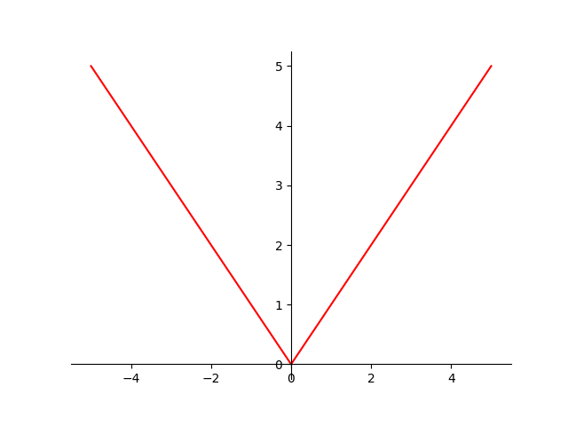
Example 9.28 (Absolute value is convex)

Let $f:\mathbb{R}\to \mathbb{R}$ be:

$$f(x)=|x|.$$

with $\mathrm{dom}f=\mathbb{R}$.

Recall that $|x|$ is a norm on the real line $\mathbb{R}$. Thus, it satisfies the triangle inequality:

$$|x+y|\le |x|+|y|\mathrm{\forall }x,y\in \mathbb{R}.$$

In particular, for any $t\in [0,1]$

$$|tx+(1-t)y|\le |tx|+|(1-t)y|=|t||x|+|1-t||y|=t|x|+(1-t)|y|.$$

Thus $f$ satisfies the convexity defining inequality (9.1):

$$f(tx+(1-t)y)\le tf(x)+(1-t)f(y)\mathrm{\forall }x,y\in \mathbb{R}.$$

Hence, $f$ is convex.

9.8.1.6. Norms

Theorem 9.69 (All norms are convex)

Let $\Vert \cdot \Vert :\mathbb{V}\to \mathbb{R}$ be a norm on a real vector space $\mathbb{V}$. Then, it satisfies the triangle inequality:

$$\Vert \mathbf{x}+\mathbf{y}\Vert \le \Vert \mathbf{x}\Vert +\Vert \mathbf{y}\Vert \mathrm{\forall }\mathbf{x},\mathbf{y}\in \mathbb{V}.$$

In particular, for any $t\in [0,1]$

$$\Vert t\mathbf{x}+(1-t)\mathbf{y}\Vert \le \Vert t\mathbf{x}\Vert +\Vert (1-t)\mathbf{y}\Vert =|t|\Vert \mathbf{x}\Vert +|1-t|\Vert \mathbf{y}\Vert =t\Vert \mathbf{x}\Vert +(1-t)\Vert \mathbf{y}\Vert .$$

Thus $f$ satisfies the convexity defining inequality (9.1). Hence, $f$ is convex.

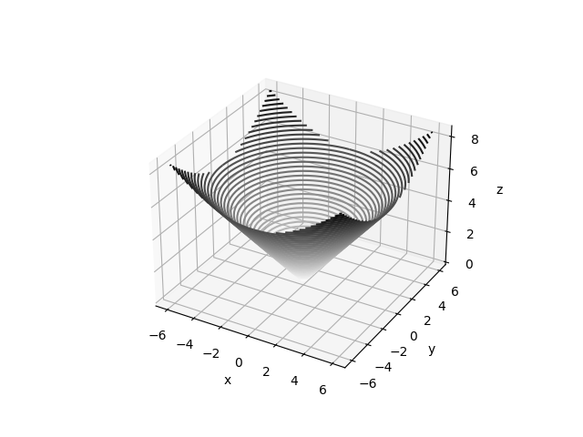
Fig. 9.4 ${\ell }_2$ norm for ${\mathbb{R}}^2$. $\Vert \cdot {\Vert }_2:{\mathbb{R}}^2\to \mathbb{R}$ 3D contour plots.

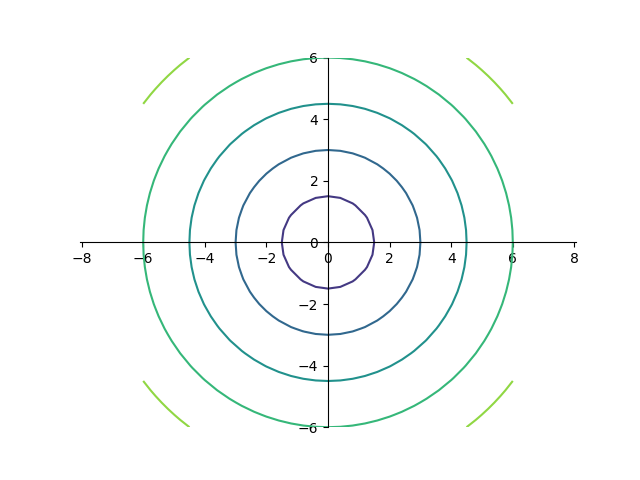
Fig. 9.5 ${\ell }_2$ norm for ${\mathbb{R}}^2$. $\Vert \cdot {\Vert }_2:{\mathbb{R}}^2\to \mathbb{R}$ 2D contour plots.

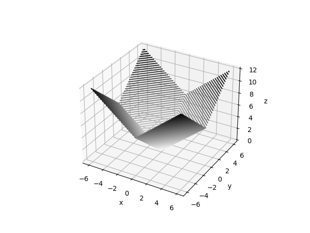
Fig. 9.6 ${\ell }_1$ norm for ${\mathbb{R}}^2$. $\Vert \cdot {\Vert }_1:{\mathbb{R}}^2\to \mathbb{R}$ 3D contour plots.

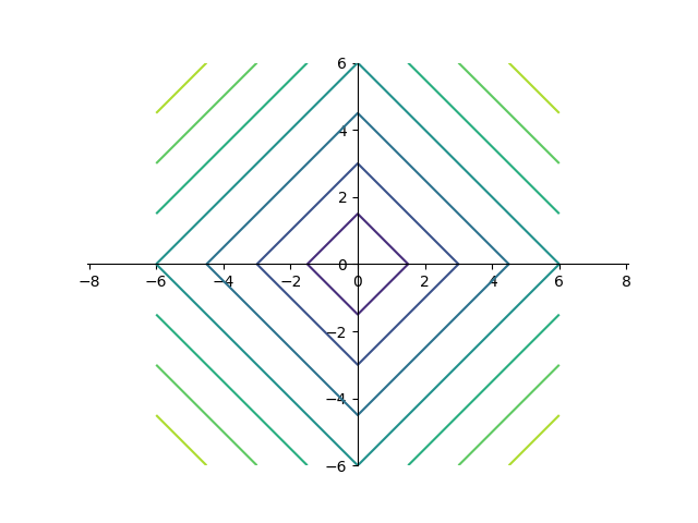
Fig. 9.7 ${\ell }_1$ norm for ${\mathbb{R}}^2$. $\Vert \cdot {\Vert }_2:{\mathbb{R}}^1\to \mathbb{R}$ 2D contour plots.

9.8.1.7. Max Function

Example 9.29 (Max function is convex)

Let $f:{\mathbb{R}}^n\to \mathbb{R}$ be:

$$f(\mathbf{x})=max\{x_1,\dots ,x_n\}.$$

with $\mathrm{dom}f={\mathbb{R}}^n$.

Let $\mathbf{x},\mathbf{y}\in {\mathbb{R}}^n$ and $t\in [0,1]$.

1. Let $x=f(\mathbf{x})=max\{x_1,\dots ,x_n\}$ and $y=f(\mathbf{y})=max\{y_1,\dots ,y_n\}$.

2. Then, for every $k=1,\dots ,n$, we have: $x_k\le x$ and $y_k\le y$.

3. Thus, $t{x}_k+(1-t)y_k\le tx+(1-t)y$.

4. Taking maximum on the left hand side, we obtain:

   $$\underset{k=1}{\overset{n}{max}}(t{x}_k+(1-t)y_k)\le tx+(1-t)y.$$

5. But $f(t\mathbf{x}+(1-t)\mathbf{y})=\underset{k=1}{\overset{n}{max}}(t{x}_k+(1-t)y_k)$.

6. Thus, $f$ satisfies the convexity defining inequality (9.1):

   $$f(t\mathbf{x}+(1-t)\mathbf{y})\le tf(\mathbf{x})+(1-t)f(\mathbf{y}).$$

7. Thus, $f$ is convex.

9.8.1.8. Geometric Mean

Example 9.30 (Geometric mean is concave)

Let $f:{\mathbb{R}}^n\to \mathbb{R}$ be given by:

$$f(\mathbf{x})={\left(\prod _{i=1}^n{x}_i\right)}^{\frac{1}{n}}$$

with $\mathrm{dom}f={\mathbb{R}}_{++}^n$.

Recall from AM-GM inequality:

$${\left(\prod _{i=1}^n{a}_i\right)}^{\frac{1}{n}}\le \frac{1}{n}\left(\sum _{i=1}^n{a}_i\right).$$

1. Let $\mathbf{x},\mathbf{y}\in {\mathbb{R}}_{++}^n$ and $t\in [0,1]$.

2. Let $\mathbf{z}=t\mathbf{x}+(1-t)\mathbf{y}$.

3. Note that $\mathbf{z}\in {\mathbb{R}}_{++}^n$ too, hence every component of $\mathbf{z}$ is positive.

4. With $a_i=\frac{x_i}{z_i}$, and applying AM-GM inequality:

   $$\frac{f(\mathbf{x})}{f(\mathbf{z})}={\left(\prod _{i=1}^n\frac{x_i}{z_i}\right)}^{\frac{1}{n}}\le \frac{1}{n}\left(\sum _{i=1}^n\frac{x_i}{z_i}\right).$$

5. With $a_i=\frac{y_i}{z_i}$, and applying AM-GM inequality:

   $$\frac{f(\mathbf{y})}{f(\mathbf{z})}={\left(\prod _{i=1}^n\frac{y_i}{z_i}\right)}^{\frac{1}{n}}\le \frac{1}{n}\left(\sum _{i=1}^n\frac{y_i}{z_i}\right).$$

6. Multiplying the first inequality by $t$ and the second by $(1-t)$ and adding them, we get:

   $$\frac{tf(\mathbf{x})+(1-t)f(\mathbf{y})}{f(\mathbf{z})}\le \frac{1}{n}(\sum _{i=1}^n\frac{t{x}_i}{z_i}+\frac{(1-t)y_i}{z_i}).$$

7. Recall that $z_i=t{x}_i+(1-t)y_i$. Thus, the inequality above simplifies to:

   $$\begin{array}{rl}& \frac{tf(\mathbf{x})+(1-t)f(\mathbf{y})}{f(\mathbf{z})}\le 1\\ & ⟺tf(\mathbf{x})+(1-t)f(\mathbf{y})\le f(\mathbf{z})=f(t\mathbf{x}+(1-t)\mathbf{y}).\end{array}$$

8. Thus, $f$ is concave.

9.8.1.9. Powers

Example 9.31 (Powers of absolute value)

Let $f:\mathbb{R}\to \mathbb{R}$ be:

$$f(x)=|x{|}^p$$

with $\mathrm{dom}f=\mathbb{R}$.

For $p=1$, the absolute value function $f(x)=|x|$ is convex.

Consider the case where $p>1$. Let $q$ be its conjugate exponent given by $\frac{1}{p}+\frac{1}{q}=1$.

Let $x,y\in \mathbb{R}$ and $s,t\in (0,1)$ with $s+t=1$.

1. By triangle inequality:

   $$|sx+ty|\le s|x|+t|y|.$$

2. We can write this as:

   $$s|x|+t|y|=\left(s^{\frac{1}{p}}|x|\right)s^{\frac{1}{q}}+\left(t^{\frac{1}{p}}|y|\right)t^{\frac{1}{q}}.$$

3. By Hölder's inequality, for some $a_1,a_2,b_1,b_2\ge 0$

   $$a_1{b}_1+a_2{b}_2\le (a_1^p+a_2^p{)}^{\frac{1}{p}}+(b_1^q+b_2^q{)}^{\frac{1}{q}}.$$

4. Let $a_1=s^{\frac{1}{p}}|x|$, $a_2=t^{\frac{1}{p}}|y|$, $b_1=s^{\frac{1}{q}}$ and $b_2=t^{\frac{1}{q}}$.

5. Applying Hölder’s inequality,

   $$|sx+ty|\le s|x|+t|y|\le (s|x{|}^p+t|y{|}^p{)}^{\frac{1}{p}}(s+t{)}^{\frac{1}{q}}=(s|x{|}^p+t|y{|}^p{)}^{\frac{1}{p}}.$$

6. Taking power of $p$ on both sides, we get:

   $$|sx+ty{|}^p\le s|x{|}^p+t|y{|}^p.$$

7. Which is the same as

   $$f(sx+ty)\le sf(x)+tf(y).$$

8. Thus, $f$ is convex.

9.8.1.10. Empty Function

Observation 9.4 (Empty function is convex)

Let $f:\mathbb{V}\to \mathbb{R}$ be such that $\mathrm{dom}f=\varnothing$. Then $f$ is convex.

Proof. The empty set $\mathrm{dom}f$ is vacuously convex. The defining inequality (9.1) is vacuously true for $f$ since its domain is empty.

This observation may sound uninteresting however it is important in the algebra of convex functions. Definition 2.48 provides definitions for sum of two partial functions and scalar multiplication with a partial function. If two convex functions $f$ and $g$ are such that $\mathrm{dom}f\cap \mathrm{dom}g=\varnothing$, then their sum $f+g$ is empty function. The observation above says that $f+g$ is still a convex function.

Jensen's inequality, discussed later in the section, generalizes the notion of convexity of a function to arbitrary convex combinations of points in its domain.

9.8.2. Convexity on Lines in Domain

Theorem 9.70 ($f$ is convex = $f$ is convex on lines in domain)

Let $\mathbb{V}$ be a real vector space. A function $f:\mathbb{V}\to \mathbb{R}$ is convex if and only if for any $\mathbf{x}\in \mathrm{dom}f$ and any $\mathbf{v}\in \mathbb{V}$, the function $g(t)=f(\mathbf{x}+t\mathbf{v})$ is convex (on its domain , $\{t\in \mathbb{R}|\mathbf{x}+t\mathbf{v}\in \mathrm{dom}f\}$).

In other words, $f$ is convex if and only if it is convex when restricted to any line that intersects its domain.

Proof. For any arbitrary $f$, and for any $\mathbf{x}\in \mathrm{dom}f,\mathbf{v}\in \mathbb{V}$
we have defined $g:\mathbb{R}\to \mathbb{R}$ as:

$$g(t)\triangleq f(\mathbf{x}+t\mathbf{v})$$

with the domain:

$$\mathrm{dom}g=\{t|\mathbf{x}+t\mathbf{v}\in \mathrm{dom}f\}.$$

Assume $f$ to be convex. To show that $g$ is convex, we need to show that $\mathrm{dom}g$ is convex and $g$ satisfies the convexity inequality.

1. Let $t_1,t_2\in \mathrm{dom}g$.

2. It means that there are $\mathbf{y}=\mathbf{x}+t_1\mathbf{v}\in \mathrm{dom}f$ and $\mathbf{z}=\mathbf{x}+t_2\mathbf{v}\in \mathrm{dom}f$,

3. and $g(t_1)=f(\mathbf{y})$ and $g(t_2)=f(\mathbf{z})$.

4. Let $r\in [0,1]$ and $t=r{t}_1+(1-r)t_2$.

5. Note that:

   $$\begin{array}{rl}\mathbf{x}+t\mathbf{v}& =\mathbf{x}+(r{t}_1+(1-r)t_2)\mathbf{v}\\ & =r\mathbf{x}+(1-r)\mathbf{x}+r{t}_1\mathbf{v}+(1-r)t_2\mathbf{v}\\ & =r(\mathbf{x}+t_1\mathbf{v})+(1-r)(\mathbf{x}+t_2\mathbf{v})\\ & =r\mathbf{y}+(1-r)\mathbf{z}.\end{array}$$

6. Since $\mathrm{dom}f$ is convex, hence $r\mathbf{y}+(1-r)\mathbf{z}\in \mathrm{dom}f$.

7. Thus, $g$ is defined at $t=r{t}_1+(1-r)t_2$ for all $r\in [0,1]$.

8. We have shown that if $t_1,t_2\in \mathrm{dom}g$, then $t=r{t}_1+(1-r)t_2\in \mathrm{dom}g$ for all $r\in [0,1]$.

9. Thus, $\mathrm{dom}g$ is convex.

10. Now,

    $$\begin{array}{rl}g(t)& =g(r{t}_1+(1-r)t_2)\\ & =f(r\mathbf{y}+(1-r)\mathbf{z})\\ & \le rf(\mathbf{y})+(1-r)f(\mathbf{z})\\ & =rg(t_1)+(1-r)g(t_2).\end{array}$$

11. We showed that for any $t_1,t_2\in \mathrm{dom}g$ and $r\in [0,1]$,

    $$g(r{t}_1+(1-r)t_2)\le rg(t_1)+(1-r)g(t_2).$$

12. Thus, $g$ is convex.

For the converse, we need to show that if for any $\mathbf{x}\in \mathrm{dom}f$ and any $\mathbf{v}\in \mathbb{V}$, $g$ is convex, then $f$ is convex.

Assume for contradiction that $f$ is not convex. Then, either $\mathrm{dom}f$ is not convex or there exists some $\mathbf{x},\mathbf{y}\in \mathrm{dom}f$ and $t\in [0,1]$ such that:

$$f((1-t)\mathbf{x}+t\mathbf{y})>(1-t)f(\mathbf{x})+tf(\mathbf{y}).$$

We show that both of these conditions lead to contradictions.

1. Assume $\mathrm{dom}f$ is not convex.

2. Then, there exists $\mathbf{x},\mathbf{y}\in \mathrm{dom}f$ such that for some $t\in [0,1]$:

   $$(1-t)\mathbf{x}+t\mathbf{y}\notin \mathrm{dom}f.$$

3. Let $\mathbf{v}=\mathbf{y}-\mathbf{x}$.

4. Note that $(1-t)\mathbf{x}+t\mathbf{y}=\mathbf{x}+t\mathbf{v}$.

5. Picking $g$ for this particular choice of $\mathbf{x}$ and $\mathbf{v}$, we note that $g$ is defined at $t=0$ and $t=1$ since they corresponding to the points $\mathbf{x}$ and $\mathbf{y}$ respectively in $\mathrm{dom}f$.

6. Since $g$ is convex by hypothesis, hence, $g$ is defined at every $t\in [0,1]$.

7. This contradicts the fact that $g$ is not defined at some $t\in [0,1]$.

8. Thus, $\mathrm{dom}f$ must be convex.

We now accept that $\mathrm{dom}f$ is convex, but there exists some $\mathbf{x},\mathbf{y}\in \mathrm{dom}f$ and $t\in [0,1]$ such that:

$$f((1-t)\mathbf{x}+t\mathbf{y})>(1-t)f(\mathbf{x})+tf(\mathbf{y}).$$

1. Again, let $\mathbf{v}=\mathbf{y}-\mathbf{x}$ and note that $(1-t)\mathbf{x}+t\mathbf{y}=\mathbf{x}+t\mathbf{v}$.

2. Pick $g$ for this choice of $\mathbf{x}$ and $\mathbf{v}$.

3. We have $g(t)=f(\mathbf{x}+t\mathbf{v})$.

4. In particular, $g(0)=f(\mathbf{x})$ and $g(1)=f(\mathbf{y})$.

5. Since $g$ is convex, hence for every $t\in [0,1]$,

   $$\begin{array}{rl}f((1-t)\mathbf{x}+t\mathbf{y})& =f(\mathbf{x}+t\mathbf{v})\\ & =g(t)\\ & =g((1-t)0+t1)\\ & \le (1-t)g(0)+tg(1)\\ & =(1-t)f(\mathbf{x})+tf(\mathbf{y}).\end{array}$$

6. We have a contradiction.

7. Thus, $f$ must be convex.

A good application of this result is in showing the concavity of the log determinant function in Example 9.49 below.

9.8.3. Epigraph

The epigraph of a function $f:\mathbb{V}\to \mathbb{R}$ is given by:

$$\mathrm{epi}f=\{(\mathbf{x},t)\in \mathbb{V}\oplus \mathbb{R}|\mathbf{x}\in \mathrm{dom}f,f(\mathbf{x})\le t\}.$$

$\mathbb{V}\oplus \mathbb{R}$ is the direct sum of $\mathbb{V}$ and $\mathbb{R}$ having appropriate vector space structure.

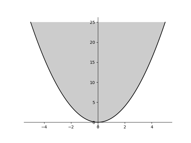
Fig. 9.8 Epigraph of the function $f(x)=x^2$.

The definition of epigraph also applies for extended real valued functions $f:\mathbb{V}\to \bar{\mathbb{R}}$.

9.8.3.1. Convex Functions

Theorem 9.71 (Function convexity = Epigraph convexity)

Let $\mathbb{V}$ be a real vector space. A function $f:\mathbb{V}\to \mathbb{R}$ is convex if and only if its epigraph $\mathrm{epi}f$ is a convex set.

This statement is also valid for extended real valued functions.

Proof. Let $C=\mathrm{epi}f$.

Assume $f$ is convex.

1. Let $({\mathbf{x}}_1,t_1),({\mathbf{x}}_2,t_2)\in \mathrm{epi}f$.

2. Then, $f({\mathbf{x}}_1)\le t_1$ and $f({\mathbf{x}}_2)\le t_2$.

3. Let $r\in [0,1]$.

4. Consider the point $(\mathbf{x},t)=r({\mathbf{x}}_1,t_1)+(1-r)({\mathbf{x}}_2,t_2)$.

5. We have $\mathbf{x}=r{\mathbf{x}}_1+(1-r)({\mathbf{x}}_2)$.

6. And $t=r{t}_1+(1-r)t_2$.

7. Then, $rf({\mathbf{x}}_1)+(1-r)f({\mathbf{x}}_2)\le r{t}_1+(1-r)t_2=t$.

8. Since $f$ is convex, hence $f(\mathbf{x})=f(r{\mathbf{x}}_1+(1-r)({\mathbf{x}}_2))\le rf({\mathbf{x}}_1)+(1-r)f({\mathbf{x}}_2)$.

9. But then, $f(\mathbf{x})\le t$.

10. Thus, $(\mathbf{x},t)\in \mathrm{epi}f$.

11. Thus, $({\mathbf{x}}_1,t_1),({\mathbf{x}}_2,t_2)\in \mathrm{epi}f$ implies $r({\mathbf{x}}_1,t_1)+(1-r)({\mathbf{x}}_2,t_2)\in \mathrm{epi}f$ for all $r\in [0,1]$.

12. Thus, $\mathrm{epi}f$ is convex.

Assume $\mathrm{epi}f$ is convex.

1. Let ${\mathbf{x}}_1,{\mathbf{x}}_2\in \mathrm{dom}f$.

2. Let $t_1=f({\mathbf{x}}_1)$ and $t_2=f({\mathbf{x}}_2)$.

3. Then, $({\mathbf{x}}_1,t_1),({\mathbf{x}}_2,t_2)\in \mathrm{epi}f$.

4. Let $r\in [0,1]$.

5. Let $\mathbf{x}=r{\mathbf{x}}_1+(1-r){\mathbf{x}}_2$.

6. Since $\mathrm{epi}f$ is convex, hence $r({\mathbf{x}}_1,t_1)+(1-r)({\mathbf{x}}_2,t_2)\in \mathrm{epi}f$.

7. i.e., $(r{\mathbf{x}}_1+(1-r){\mathbf{x}}_2,r{t}_1+(1-r)t_2)\in \mathrm{epi}f$.

8. Thus, $\mathbf{x}=r{\mathbf{x}}_1+(1-r){\mathbf{x}}_2\in \mathrm{dom}f$.

9. Thus, $\mathrm{dom}f$ is convex.

10. And, $f(\mathbf{x})\le r{t}_1+(1-r)t_2$.

11. But $r{t}_1+(1-r)t_2=rf({\mathbf{x}}_1)+(1-r)f({\mathbf{x}}_2)$.

12. Thus, $f(r{\mathbf{x}}_1+(1-r){\mathbf{x}}_2)\le rf({\mathbf{x}}_1)+(1-r)f({\mathbf{x}}_2)$.

13. Thus, $f$ is convex as ${\mathbf{x}}_1,{\mathbf{x}}_2\in \mathrm{dom}f$ and $r\in [0,1]$ were arbitrary.

Note that $\mathrm{dom}f$ is the projection of $\mathrm{epi}f$ from $\mathbb{V}\oplus \mathbb{R}$ to $\mathbb{V}$. Due to Theorem 9.31, $\mathrm{epi}f$ convex implies $\mathrm{dom}f$ convex as the projection is a linear operation.

Theorem 9.72 (Convex function from convex set by minimization)

Let $C$ be a nonempty convex set in $\mathbb{V}\oplus \mathbb{R}$. Let $f:\mathbb{V}\to \bar{\mathbb{R}}$ be the function defined by

$$f(\mathbf{x})=inf\{w\in \mathbb{R}|(\mathbf{x},w)\in C\}\mathrm{\forall }\mathbf{x}\in \mathbb{V}.$$

Then $f$ is convex.

Proof. We show the convexity of $f$ by showing the convexity of its epigraph.

1. Let $(\mathbf{x},s)$ and $(\mathbf{y},t)$ be two points in $\mathrm{epi}f$.

2. Then $f(\mathbf{x})\le s$ and $f(\mathbf{y})\le t$.

3. By the definition of $f$ (infimum rule), for every $k\in \mathbb{N}$, there exists $(\mathbf{x},s_k)\in C$ such that $s_k\le s+\frac{1}{k}$.

4. Similarly, for every $k\in \mathbb{N}$, there exists $(\mathbf{y},t_k)\in C$ such that $t_k\le t+\frac{1}{k}$.

5. Consider the sequences $\{(\mathbf{x},s_k)\}$ and $\{(\mathbf{y},t_k)\}$.

6. By the convexity of $C$, for every $r\in [0,1]$ and every $k$

   $$(r\mathbf{x}+(1-r)\mathbf{y},r{s}_k+(1-r)t_k)\in C.$$

7. Hence for every $k$

   $$f(r\mathbf{x}+(1-r)\mathbf{y})\le r{s}_k+(1-r)t_k.$$

8. Taking the limit $k\to \mathrm{\infty }$, we have

   $$f(r\mathbf{x}+(1-r)\mathbf{y})\le rs+(1-r)t.$$

9. Hence $(r\mathbf{x}+(1-r)\mathbf{y},rs+(1-r)t)\in \mathrm{epi}f$ for every $r\in [0,1]$.

10. Hence $\mathrm{epi}f$ is convex.

11. Hence $f$ is convex.

9.8.3.2. Nonnegative Homogeneous Functions

Recall that a real valued function $f:\mathbb{V}\to \mathbb{R}$ is nonnegative homogeneous if for every $t\in {\mathbb{R}}_{+}$, $f(t\mathbf{x})=tf(\mathbf{x})$.

Theorem 9.73 (Nonnegative homogeneity = Epigraph is cone)

A function $f:\mathbb{V}\to \mathbb{R}$ is nonnegative homogeneous if and only if its epigraph $\mathrm{epi}f$ is a cone in $\mathbb{V}\oplus \mathbb{R}$.

Proof. Let $f$ be nonnegative homogeneous.

1. Let $(\mathbf{x},f(\mathbf{x}))\in \mathrm{epi}f$.

2. Let $t\ge 0$.

3. Then, $t(\mathbf{x},f(\mathbf{x}))=(t\mathbf{x},tf(\mathbf{x}))=(t\mathbf{x},f(t\mathbf{x}))$.

4. But $(t\mathbf{x},f(t\mathbf{x}))\in \mathrm{epi}f$ since $f$ is nonnegative homogeneous.

5. Thus, $\mathbb{V}\oplus \mathbb{R}$ is closed under nonnegative scalar multiplication.

6. Thus, $\mathrm{epi}f$ is a cone.

Assume $\mathrm{epi}f$ is a cone.

1. Let $\mathbf{x}\in \mathrm{dom}f$.

2. Then, $(\mathbf{x},f(\mathbf{x}))\in \mathrm{epi}f$.

3. Since $(\mathbf{0},0)\in \mathrm{epi}f$ as $\mathrm{epi}f$ is a cone, hence $f(0\mathbf{x})=0f(\mathbf{x})=0$.

4. Now, let $t>0$.

5. Since $\mathrm{epi}f$ is a cone then, $t(\mathbf{x},f(\mathbf{x}))\in \mathrm{epi}f$.

6. Then, $t(\mathbf{x},f(\mathbf{x}))=(t\mathbf{x},tf(\mathbf{x}))\in \mathrm{epi}f$.

7. By definition of epigraph, $f(t\mathbf{x})\le tf(\mathbf{x})$.

8. We claim that $f(t\mathbf{x})=tf(\mathbf{x})$ must hold true.

9. Assume for contradiction that $f(t\mathbf{x})=sf(\mathbf{x})$ where $s<t$.

10. Then, $(t\mathbf{x},sf(\mathbf{x}))\in \mathrm{epi}f$.

11. Since $\mathrm{epi}f$ is a cone, hence dividing by $t$, we get, $(\mathbf{x},\frac{s}{t}f(\mathbf{x}))\in \mathrm{epi}f$.

12. But then, $f(\mathbf{x})\le \frac{s}{t}f(\mathbf{x})<f(\mathbf{x})$ which is a contradiction.

13. Hence, $f(t\mathbf{x})=tf(\mathbf{x})$ must hold true.

9.8.3.3. Nonnegative Homogeneous Convex Functions

Theorem 9.74 (Nonnegative homogeneous convex function epigraph characterization)

Let $\mathbb{V}$ be a real vector space. A real valued function $f:\mathbb{V}\to \mathbb{R}$ is nonnegative homogeneous and convex if and only if its epigraph $\mathrm{epi}f$ is a convex cone.

Proof. By Theorem 9.73, $f$ is nonnegative homogeneous if and only if $\mathrm{epi}f$ is a cone.

By Theorem 9.71, $f$ is convex if and only if $\mathrm{epi}f$ is convex.

Thus, $f$ is nonnegative homogeneous and convex if and only if its epigraph $\mathrm{epi}f$ is a convex cone.

Theorem 9.75 (Nonnegative homogeneous convex function is subadditive)

Let $\mathbb{V}$ be a real vector space. A nonnegative homogeneous function $f:\mathbb{V}\to \mathbb{R}$ is convex if and only if it is subadditive:

$$f(\mathbf{x}+\mathbf{y})\le f(\mathbf{x})+f(\mathbf{y})\mathrm{\forall }\mathbf{x},\mathbf{y}\in \mathrm{dom}f.$$

Proof. Assume that $f$ is nonnegative homogeneous and convex.

1. By Theorem 9.74, $\mathrm{epi}f$ is a convex cone.

2. Then, by Theorem 9.47 $\mathrm{epi}f$ is closed under addition and nonnegative scalar multiplication.

3. Pick any $\mathbf{x},\mathbf{y}\in \mathrm{dom}f$.

4. Then $(\mathbf{x},f(\mathbf{x})),(\mathbf{y},f(\mathbf{y}))\in \mathrm{epi}f$.

5. Then, their sum $(\mathbf{x}+\mathbf{y},f(\mathbf{x})+f(\mathbf{y}))\in \mathrm{epi}f$.

6. This means that $f(\mathbf{x}+\mathbf{y})\le f(\mathbf{x})+f(\mathbf{y})$ by definition of epigraph.

Now for the converse, assume that $f$ is nonnegative homogeneous and subadditive.

1. By Theorem 9.73, $\mathrm{epi}f$ is a cone.

2. Consequently, it is closed under nonnegative scalar multiplication.

3. Pick any $\mathbf{x},\mathbf{y}\in \mathrm{dom}f$.

4. Let $(\mathbf{x},\alpha ),(\mathbf{y},\beta )\in \mathrm{epi}f$.

5. Then, $f(\mathbf{x})\le \alpha$ and $f(\mathbf{y})\le \beta$.

6. Now, $(\mathbf{x}+\mathbf{y},f(\mathbf{x}+\mathbf{y}))\in \mathrm{epi}f$.

7. Since $f$ is subadditive, hence $f(\mathbf{x}+\mathbf{y})\le f(\mathbf{x})+f(\mathbf{y})\le \alpha +\beta$.

8. Thus, $(\mathbf{x}+\mathbf{y},\alpha +\beta )\in \mathrm{epi}f$.

9. We have shown that for any $(\mathbf{x},\alpha ),(\mathbf{y},\beta )\in \mathrm{epi}f$, $(\mathbf{x}+\mathbf{y},\alpha +\beta )\in \mathrm{epi}f$.

10. Thus, $\mathrm{epi}f$ is closed under vector addition.

11. Since $\mathrm{epi}f$ is closed under vector addition and nonnegative scalar multiplication, hence $\mathrm{epi}f$ is a convex cone.

12. But then, by Theorem 9.74, $f$ is convex.

Corollary 9.5

Let $\mathbb{V}$ be a real vector space. Let $f:\mathbb{V}\to \mathbb{R}$ be a nonnegative homogeneous convex function. Then,

$$f(-\mathbf{x})\ge -f(\mathbf{x})\mathrm{\forall }\mathbf{x}\in \mathrm{dom}f.$$

Proof. Since $f$ is nonnegative homogeneous convex, hence $f$ is subadditive.

Thus,

$$f(\mathbf{x}-\mathbf{x})\le f(\mathbf{x})+f(-\mathbf{x}).$$

But,

$$f(\mathbf{x}-\mathbf{x})=f(\mathbf{0})=f(0\mathbf{0})=0f(\mathbf{0})=0.$$

Thus,

$$f(\mathbf{x})+f(-\mathbf{x})\ge 0.$$

Thus,

$$f(-\mathbf{x})\ge -f(\mathbf{x}).$$

Theorem 9.76 (Linearity of nonnegative homogeneous functions)

Let $\mathbb{V}$ be a real vector space. Let $f:\mathbb{V}\to \mathbb{R}$ be a nonnegative homogeneous convex function. Then, $f$ is linear on a subspace $L$ of $\mathbb{V}$ if and only if $f(-\mathbf{x})=-f(\mathbf{x})$ for every $\mathbf{x}\in L$.

If $L$ is finite dimensional, then this is true if merely $f(-{\mathbf{b}}_i)=-f({\mathbf{b}}_i)$ for all the vectors in some basis ${\mathbf{b}}_1,\dots ,{\mathbf{b}}_n$ for $L$.

Proof. We are given that $f$ is nonnegative homogeneous convex.

Assume that $f$ is linear over $L$. Then by definition of linearity, $f(-\mathbf{x})=-f(\mathbf{x})$ for every $\mathbf{x}\in L$.

Now, for the converse, assume that $f(-\mathbf{x})=-f(\mathbf{x})\mathrm{\forall }\mathbf{x}\in L$.

1. Let $\mathbf{x},\mathbf{y}\in L$.

2. Then, $f(\mathbf{x}+\mathbf{y})\le f(\mathbf{x})+f(\mathbf{y})$ since $f$ is subadditive.

3. Also,

   $$f(\mathbf{x}+\mathbf{y})=-f(-(\mathbf{x}+\mathbf{y}))=-f(-\mathbf{x}+(-\mathbf{y})).$$

4. But

   $$f(-\mathbf{x}+(-\mathbf{y}))\le f(-\mathbf{x})+f(-\mathbf{y})=-f(\mathbf{x})-f(\mathbf{y})=-(f(\mathbf{x})+f(\mathbf{y})).$$

5. Thus,

   $$f(\mathbf{x}+\mathbf{y})=-f(-\mathbf{x}+(-\mathbf{y}))\ge f(\mathbf{x})+f(\mathbf{y}).$$

6. Combining, we get $f(\mathbf{x}+\mathbf{y})=f(\mathbf{x})+f(\mathbf{y})$. Thus, $f$ is additive over $L$.

7. For any $t<0$,

   $$f(t\mathbf{x})=-f(-t\mathbf{x})=-(-t)f(\mathbf{x})=tf(\mathbf{x}).$$

8. Thus, for any $t\in \mathbb{R}$, $f(t\mathbf{x})=tf(\mathbf{x})$.

9. Thus, $f$ is homogeneous over $L$.

10. Since $f$ is additive and homogeneous over $L$, hence $f$ is linear.

Finally, assume that $L$ is finite dimensional and has a basis ${\mathbf{b}}_1,\dots ,{\mathbf{b}}_n$.

1. By previous argument $f$ is homogeneous on the basis vectors; i.e., $f(t{\mathbf{b}}_i)=tf({\mathbf{b}}_i)$ for any $t\in \mathbb{R}$ and any basis vector.

2. Let $\mathbf{x}\in L$.

3. Then, $\mathbf{x}=\sum _{i=1}^n{a}_i{\mathbf{b}}_i$.

4. Since $f$ is subadditive, hence

   $$\begin{array}{rl}f(a_1{\mathbf{b}}_1)+\cdots +f(a_n{\mathbf{b}}_n)& \ge f(a_1{\mathbf{b}}_1+\cdots +a_n{\mathbf{b}}_n)\\ & =f(\mathbf{x})\\ & \ge -f(-\mathbf{x})\\ & =-f(-a_1{\mathbf{b}}_1-\cdots -a_n{\mathbf{b}}_n)\\ & \ge -f(-a_1{\mathbf{b}}_1)-\cdots -f(-a_n{\mathbf{b}}_n)\\ & =f(a_1{\mathbf{b}}_1)+\cdots +f(a_n{\mathbf{b}}_n).\end{array}$$

5. This can hold only if all the inequalities are equalities in the previous derivation.

6. Thus, $f(\mathbf{x})=-f(-\mathbf{x})$ or $-f(\mathbf{x})=f(-\mathbf{x})$ for every $\mathbf{x}\in L$.

7. Then, following the previous argument, $f$ is linear over $L$.

9.8.4. Extended Value Extensions

Tracking domains of convex functions is difficult. It is often convenient to extend a convex function $f:\mathbb{V}\to \mathbb{R}$ with a domain $\mathrm{dom}f\subset \mathbb{V}$ to all of $\mathbb{V}$ by defining it to be $\mathrm{\infty }$ outside its domain.

Definition 9.46 (Extended value extension)

The extended value extension of a convex function $f:\mathbb{V}\to \mathbb{R}$ is defined as $\tilde{f}:\mathbb{V}\to \bar{\mathbb{R}}$ given by:

$$\begin{array}{r}\tilde{f}(\mathbf{x})\triangleq \{\begin{array}{lll}f(\mathbf{x})& \text{for}& \mathbf{x}\in \mathrm{dom}f\\ \mathrm{\infty }& \text{for}& \mathbf{x}\notin \mathrm{dom}f.\end{array}\end{array}$$

We mention that the defining inequality (9.1) for a convex function $f$ remains valid (rather gets extended) for its extended value extension too. If $f$ is convex over $\mathrm{dom}f$, then for any ${\mathbf{x}}_1,{\mathbf{x}}_2\in \mathbb{V}$, and $0<t<1$, we have

$$\tilde{f}(t{\mathbf{x}}_1+(1-t){\mathbf{x}}_2)\le t\tilde{f}({\mathbf{x}}_1)+(1-t)\tilde{f}({\mathbf{x}}_2).$$

1. At $t=0$ and $t=1$, this is always an equality.

2. Since $\mathrm{dom}f$ is convex, hence if both ${\mathbf{x}}_1,{\mathbf{x}}_2\in \mathrm{dom}f$, then $t{\mathbf{x}}_1+(1-t){\mathbf{x}}_2\in \mathrm{dom}f$ too.

3. The inequality then reduces to (9.1).

4. If either ${\mathbf{x}}_1$ or ${\mathbf{x}}_2$ is not in $\mathrm{dom}f$, then the R.H.S. becomes $\mathrm{\infty }$ and the inequality stays valid.

Definition 9.47 (Effective domain)

The effective domain of an extended valued function $\tilde{f}:\mathbb{V}\to \bar{\mathbb{R}}$ is defined as:

$$\mathrm{dom}\tilde{f}=\{\mathbf{x}\in \mathbb{V}|\tilde{f}(\mathbf{x})<\mathrm{\infty }\}.$$

An equivalent way to define the effective domain is:

$$\mathrm{dom}\tilde{f}=\{\mathbf{x}\in \mathbb{V}|\mathrm{\exists }t\in \mathbb{R}\text{ with }(\mathbf{x},t)\in \mathrm{epi}f\}.$$

Theorem 9.77 (Effective domain and sum of functions)

If $f$ and $g$ are two extended valued functions, then $\mathrm{dom}(f+g)=\mathrm{dom}f\cap \mathrm{dom}g$.

Proof. We proceed as follows:

1. At any $\mathbf{x}\in \mathrm{dom}f\cap \mathrm{dom}g$, both $f(\mathbf{x})$ and $g(\mathbf{x})$ are finite.

2. Thus, $f(\mathbf{x})+g(\mathbf{x})$ is finite.

3. Hence, $\mathbf{x}\in \mathrm{dom}(f+g)$.

4. At any $\mathbf{x}\in \mathbb{V}\setminus (\mathrm{dom}f\cap \mathrm{dom}g)$, either $f(\mathbf{x})=\mathrm{\infty }$ or $g(\mathbf{x})=\mathrm{\infty }$.

5. Thus, $(f+g)(\mathbf{x})=f(\mathbf{x})+g(\mathbf{x})=\mathrm{\infty }$.

6. Thus, $\mathbf{x}\notin \mathrm{dom}(f+g)$.

Several commonly used convex functions have vastly different domains. If we work with these functions directly, then we have to constantly worry about identifying the domain and manipulating the domain as per the requirements of the operations we are considering. This quickly becomes tedious.

An alternative approach is to work with the extended value extensions of all functions. We don’t have to worry about tracking the function domain. The domain can be identified whenever needed by removing the parts from $\mathbb{V}$ where the function goes to $\mathrm{\infty }$.

In this book, unless otherwise specified, we shall assume that the functions are being treated as their extended value extensions.

9.8.5. Proper Functions

Definition 9.48 (Proper function)

An extended real-valued function $f:\mathbb{V}\to \bar{\mathbb{R}}$ is called proper if its domain is nonempty, it never takes the value $-\mathrm{\infty }$ and is not identically equal to $\mathrm{\infty }$.

$$\mathrm{\exists }\mathbf{x}\in \mathbb{V}\text{ such that }f(\mathbf{x})<\mathrm{\infty }\text{ and }f(\mathbf{x})>-\mathrm{\infty }\mathrm{\forall }\mathbf{x}\in \mathbb{V}.$$

In other words, $\mathrm{epi}f$ is nonempty and contains no vertical lines.

Putting another way, a proper function is obtained by taking a real valued function $f$ defined on a nonempty set $C\subseteq \mathbb{V}$ and then extending it to all of $\mathbb{V}$ by setting $f(\mathbf{x})=+\mathrm{\infty }$ for all $\mathbf{x}\notin C$.

It is easy to see that the codomain for a proper function can be changed from $\bar{\mathbb{R}}$ to $(-\mathrm{\infty },\mathrm{\infty }]$ to clarify that it never takes the value $-\mathrm{\infty }$.

Definition 9.49 (Improper function)

An extended real-valued function $f:\mathbb{V}\to \bar{\mathbb{R}}$ is called improper if it is not proper.

For an improper function $f$:

• $\mathrm{dom}f$ may be empty.

• $f$ might take a value of $-\mathrm{\infty }$ at some $\mathbf{x}\in \mathbb{V}$.

Most of our study is focused on proper functions. However, improper functions sometimes do arise naturally in convex analysis.

Example 9.32 (An improper function)

Consider a function $f:\mathbb{R}\to \bar{\mathbb{R}}$ as described below:

$$\begin{array}{r}f(x)=\{\begin{array}{lll}-\mathrm{\infty }& \text{ if }& |x|<1\\ 0& \text{ if }& |x|=1\\ \mathrm{\infty }& \text{ if }& |x|>1.\end{array}\end{array}$$

Then, $f$ is an improper function.

9.8.6. Indicator Functions

Definition 9.50 (Indicator function)

Let $C\subseteq \mathbb{V}$. Then, its indicator function is given by $I_C(\mathbf{x})=0\mathrm{\forall }\mathbf{x}\in C$. Here, $\mathrm{dom}{I}_C=C$.

The extended value extension of an indicator function is given by:

$$\begin{array}{r}\widetilde{I_C}(\mathbf{x})\triangleq \{\begin{array}{lll}0& \text{for}& \mathbf{x}\in C\\ \mathrm{\infty }& \text{for}& \mathbf{x}\notin C.\end{array}\end{array}$$

Theorem 9.78 (Indicator functions and convexity)

An indicator function is convex if and only if its domain is a convex set.

Proof. Let $C$ be convex. Let $I_C$ be its indicator function. Let $\mathbf{x},\mathbf{y}\in C$. Then, for any $t\in [0,1]$

$$I_C(t\mathbf{x}+(1-t)\mathbf{y})=0\le t{I}_C(\mathbf{x})+(1-t)I_C(\mathbf{x})=0.$$

since $t\mathbf{x}+(1-t)\mathbf{y}\in C$ as $C$ is convex.

Thus, $I_C$ is convex.

If $C$ is not convex, then $\mathrm{dom}{I}_C$ is not convex. Hence, $I_C$ is not convex.

Theorem 9.79 (Restricting the domain of a function)

Let $f$ be a proper function. Then,

$$\mathrm{dom}(f+I_C)=\mathrm{dom}f\cap C.$$

Also,

$$(f+I_C)(\mathbf{x})=f(\mathbf{x})\mathrm{\forall }\mathbf{x}\in \mathrm{dom}f\cap C.$$

The statement is obvious. And quite powerful.

• The problem of minimizing a function $f$ over a set $C$ is same as minimizing $f+I_C$ over $\mathbb{V}$.

9.8.7. Sublevel Sets

Recall from Definition 2.53 that the $\alpha$-sublevel set for a real valued function $f:\mathbb{V}\to \mathbb{R}$ is given by

$$C_{\alpha }=\{\mathbf{x}\in \mathrm{dom}f|f(\mathbf{x})\le \alpha \}.$$

The strict sublevel sets for a real valued function $f:\mathbb{V}\to \mathbb{R}$ can be defined as

$$O_{\alpha }=\{\mathbf{x}\in \mathrm{dom}f|f(\mathbf{x})<\alpha \}.$$

The sublevel sets can be shown to be intersection of a set of strict sublevel sets.

Theorem 9.80 (Sublevel set as intersection)

Let $\mathbb{V}$ be a real vector space. Let $f:\mathbb{V}\to \mathbb{R}$ be a real valued function. Let

$$O_{\alpha }=\{\mathbf{x}\in \mathrm{dom}f|f(\mathbf{x})<\alpha \}$$

denote the strict sublevel set of $f$ for $\alpha$. Let

$$C_{\alpha }=\{\mathbf{x}\in \mathrm{dom}f|f(\mathbf{x})\le \alpha \}$$

denote the sublevel set of $f$ for $\alpha$. Then,

$$C_{\alpha }=\bigcap _{\mu >\alpha }{O}_{\mu }.$$

Proof. We show that $C_{\alpha }\subseteq \bigcap _{\mu >\alpha }{O}_{\mu }$.

1. Let $\mathbf{x}\in C_{\alpha }$.

2. Then, $f(\mathbf{x})\le \alpha$.

3. Thus, $f(\mathbf{x})<\mu$ for every $\mu >\alpha$.

4. Thus, $\mathbf{x}\in O_{\mu }$ for every $\mu >\alpha$.

5. Thus, $C_{\alpha }\subseteq \bigcap _{\mu >\alpha }{O}_{\mu }$.

We now show that $C_{\alpha }\supseteq \bigcap _{\mu >\alpha }{O}_{\mu }$.

1. Let $\mathbf{x}\in \bigcap _{\mu >\alpha }{O}_{\mu }$.

2. Then, $f(\mathbf{x})<\mu$ for every $\mu >\alpha$.

3. Taking the infimum on the R.H.S. over the set $\{\mu \in \mathbb{R}|\mu >\alpha \}$, we obtain

   $$f(\mathbf{x})\le inf\{\mu \in \mathbb{R}|\mu >\alpha \}=\alpha .$$

4. Thus, $\mathbf{x}\in C_{\alpha }$.

5. Thus, $\bigcap _{\mu >\alpha }{O}_{\mu }\subseteq C_{\alpha }$.

Theorem 9.81 (Convexity of sublevel sets)

If $f:\mathbb{V}\to \mathbb{R}$ is convex, then its sublevel sets given by

$$C_{\alpha }=\{\mathbf{x}\in \mathrm{dom}f|f(\mathbf{x})\le \alpha \}$$

are convex.

Proof. Assume $f$ is convex.

1. Let $\mathbf{x},\mathbf{y}\in C_{\alpha }$.

2. Then, $f(\mathbf{x})\le \alpha$ and $f(\mathbf{y})\le \alpha$.

3. Let $t\in [0,1]$.

4. Let $\mathbf{z}=t\mathbf{x}+(1-t)\mathbf{y}$.

5. Since $f$ is convex, hence:

   $$f(\mathbf{z})\le tf(\mathbf{x})+(1-t)f(\mathbf{y})\le t\alpha +(1-t)\alpha =\alpha .$$

6. Thus, $f(\mathbf{z})\le \alpha$.

7. Thus, $\mathbf{z}\in C_{\alpha }$.

8. Thus, $C_{\alpha }$ is convex.

The converse is not true. A function need not be convex even if all its sublevel sets are convex.

Example 9.33

Consider the function $f(x)=\ln x$. It is concave (Example 9.45).

Its sublevel sets are convex as they are intervals.

Theorem 9.82 (Convexity of strict sublevel sets)

If $f:\mathbb{V}\to \mathbb{R}$ is convex, then its strict sublevel sets given by

$$O_{\alpha }=\{\mathbf{x}\in \mathrm{dom}f|f(\mathbf{x})<\alpha \}$$

are convex.

Proof. Assume $f$ is convex.

1. Let $\mathbf{x},\mathbf{y}\in O_{\alpha }$.

2. Then, $f(\mathbf{x})<\alpha$ and $f(\mathbf{y})<\alpha$.

3. Let $t\in (0,1)$.

4. Let $\mathbf{z}=t\mathbf{x}+(1-t)\mathbf{y}$.

5. Since $f$ is convex, hence:

   $$f(\mathbf{z})\le tf(\mathbf{x})+(1-t)f(\mathbf{y})<t\alpha +(1-t)\alpha =\alpha .$$

6. Thus, $f(\mathbf{z})<\alpha$.

7. Thus, $\mathbf{z}\in O_{\alpha }$.

8. Thus, $O_{\alpha }$ is convex.

An alternate proof for showing the convexity of the sublevel sets is to show it as an intersection of strict sublevel sets.

Theorem 9.83 (Intersection of sublevel sets of convex functions)

Let $\mathbb{V}$ be a real vector space. Let $I$ be an arbitrary index set. Let $f_i:\mathbb{V}\to (-\mathrm{\infty },\mathrm{\infty }]$ be convex functions for every $i\in I$. Let ${\alpha }_i\in \mathbb{R}$ for every $i\in I$. Then,

$$C=\{\mathbf{x}|f_i(\mathbf{x})\le {\alpha }_i,\mathrm{\forall }i\in I\}$$

is a convex set.

Proof. For each $i\in I$, consider the set

$$C_i=\{\mathbf{x}|f_i(\mathbf{x})\le {\alpha }_i\}.$$

Then, $C_i$ is a sublevel set of $f_i$ which is convex. Hence, $C_i$ is convex. Now, we can see that

$$C=\bigcap _{i\in I}{C}_i$$

Thus, $C$ is an intersection of convex sets. Hence, $C$ is convex.

Example 9.34 (Convexity of sublevel sets of the quadratic)

Let $\mathbf{Q}\in {\mathbb{S}}^n$ be a positive semidefinite matrix. Let $\mathbf{a}\in {\mathbb{R}}^n$ and $c\in \mathbb{R}$.

Consider the sets of the form

$$\{\mathbf{x}\in {\mathbb{R}}^n|\frac{1}{2}⟨\mathbf{x},\mathbf{Q}\mathbf{x}⟩+⟨\mathbf{x},\mathbf{a}⟩+c\le 0\}.$$

This is a sublevel set of the quadratic function $f(\mathbf{x})=\frac{1}{2}⟨\mathbf{x},\mathbf{Q}\mathbf{x}⟩+⟨\mathbf{x},\mathbf{a}⟩+c$.

Since $f$ is convex, hence the set is convex.

Sets of this form include the solid ellipsoids, paraboloids as well as spherical balls. Here is an example of the spherical ball of the norm induced by the inner product.

$$\{\mathbf{x}|\Vert \mathbf{x}\Vert \le 1\}=\{\mathbf{x}|⟨\mathbf{x},\mathbf{x}⟩-1\le 0\}.$$

9.8.8. Hypograph

The hypograph of a function $f:\mathbb{V}\to \mathbb{R}$ is given by:

$$\mathrm{hypo}f=\{(\mathbf{x},t)\in \mathbb{V}\oplus \mathbb{R}|\mathbf{x}\in \mathrm{dom}f,f(\mathbf{x})\ge t\}.$$

Just like function convexity is connected to epigraph convexity, similarly function concavity is connected to hypograph convexity.

Theorem 9.84 (Function concavity = Hypograph convexity)

A function $f$ is concave if and only if its hypograph $\mathrm{hypo}f$ is a convex set.

Proof. $f$ is concave if and only if $-f$ is convex if and only if the epigraph of $-f$ is convex if and only if the hypograph of $f$ is convex.

9.8.9. Super-level Sets

Recall from Definition 2.56 that the $\alpha$-sublevel set for a real valued function $f:\mathbb{V}\to \mathbb{R}$ is given by

$$D_{\alpha }=\{\mathbf{x}\in \mathrm{dom}f|f(\mathbf{x})\ge \alpha \}.$$

Theorem 9.85

If $f:\mathbb{V}\to \mathbb{R}$ is concave, then its super-level sets are convex.

Proof. Assume $f$ is concave.

1. Let $\mathbf{x},\mathbf{y}\in D_{\alpha }$.

2. Then, $f(\mathbf{x})\ge \alpha$ and $f(\mathbf{y})\ge \alpha$.

3. Let $t\in [0,1]$.

4. Let $\mathbf{z}=t\mathbf{x}+(1-t)\mathbf{y}$.

5. Since $f$ is concave, hence:

   $$f(\mathbf{z})\ge tf(\mathbf{x})+(1-t)f(\mathbf{y})\ge t\alpha +(1-t)\alpha =\alpha .$$

6. Thus, $f(\mathbf{z})\ge \alpha$.

7. Thus, $\mathbf{z}\in D_{\alpha }$.

8. Thus, $D_{\alpha }$ is convex.

The converse is not true. A function need not be concave even if all its super-level sets are convex.

Example 9.35

Let geometric mean be given by:

$$g(\mathbf{x})={\left(\prod _{i=1}^n{x}_i\right)}^{\frac{1}{n}}$$

with $\mathrm{dom}g={\mathbb{R}}_{+}^n$ (with the interpretation that $0^{\frac{1}{n}}=0$).

Let arithmetic mean be given by:

$$a(\mathbf{x})=\frac{1}{n}\sum _{i=1}^n{x}_i.$$

Consider the set:

$$A=\{\mathbf{x}\in {\mathbb{R}}_{+}^n|g(\mathbf{x})\ge \alpha a(\mathbf{x})\}.$$

$A$ is the set of nonnegative vectors where the geometric mean of the components is at least $\alpha$ times larger than the arithmetic mean.

1. In Example 9.30 we establish that $g$ is concave.

2. In Example 9.26 we established that $a$ is convex as well as concave.

3. Thus, $-\alpha a$ is concave.

4. Thus, $g-\alpha a$ is concave (with $\mathrm{dom}g-\alpha a={\mathbb{R}}_{+}^n$).

5. Note that $A$ can be redefined as:

   $$A=\{\mathbf{x}\in {\mathbb{R}}_{+}^n|g(\mathbf{x})-\alpha a(\mathbf{x})\ge 0\}.$$

6. Thus, $A$ is a $0$-super-level set of $g-\alpha a$.

7. Since $g-\alpha a$ is concave, hence $A$ is convex.

9.8.10. Closed Convex Functions

Recall from Real Valued Functions that a function is closed if all its sublevel sets are closed. A function is closed if and only if its epigraph is closed. A function is closed if and only if it is lower semicontinuous.

In general, if a function is continuous, then it is lower semicontinuous and hence it is closed.

In this subsection, we provide examples of convex functions which are closed.

9.8.10.1. Affine Functions

Theorem 9.86 (Affine functions are closed)

Let $f:\mathbb{V}\to \mathbb{R}$ be given by

$$f(\mathbf{x})=⟨\mathbf{x},\mathbf{a}⟩+b$$

where $\mathbf{a}\in {\mathbb{V}}^{\ast }$ and $b\in \mathbb{R}$. Then $f$ is closed.

Proof. We prove closedness by showing that the epigraph of $f$ is closed.

1. Let $\{{\mathbf{x}}_k,t_k\}$ be a converging sequence of $\mathrm{epi}f$.

2. Let $(\mathbf{x},t)=\underset{k\to \mathrm{\infty }}{lim}({\mathbf{x}}_k,t_k)$.

3. We have $f({\mathbf{x}}_k)\le t_k$ for every $k$.

4. In other words

   $$⟨{\mathbf{x}}_k,\mathbf{a}⟩+b\le t_k\mathrm{\forall }k\in \mathbb{N}.$$

5. Taking the limit on both sides, we get

   $$⟨\mathbf{x},\mathbf{a}⟩+b\le t.$$

6. Hence $f(\mathbf{x})\le t$.

7. Hence $(\mathbf{x},t)\in \mathrm{epi}f$.

8. Hence $\mathrm{epi}f$ is closed.

9.8.10.2. Norms

Theorem 9.87 (All Norms are closed)

Let $\Vert \cdot \Vert :\mathbb{V}\to \mathbb{R}$ be a norm on a real vector space $\mathbb{V}$. Then $\Vert \cdot \Vert$ is closed.

Proof. The sublevel sets are given by $S_t=\{\mathbf{x}\in \mathbb{V}|\Vert \mathbf{x}\Vert \le t\}$. They are nothing but the closed balls of radius $t$ around $\mathbf{0}$ and by definition closed. Hence all sublevel sets are closed. Thus $\Vert \cdot \Vert$ is closed.

9.8.11. Support Functions

Definition 9.51 (Support function for a set)

Let $\mathbb{V}$ be a real inner product space. Let $C$ be a subset of $\mathbb{V}$. The support function ${\sigma }_C:\mathbb{V}\to (-\mathrm{\infty },\mathrm{\infty }]$ is defined as

$${\sigma }_C(\mathbf{x})=sup\{⟨\mathbf{x},\mathbf{y}⟩|\mathbf{y}\in C\}.$$

Since $\mathbb{V}$ and ${\mathbb{V}}^{\ast }$ are isomorphic, support function ${\sigma }_C:{\mathbb{V}}^{\ast }\to (-\mathrm{\infty },\mathrm{\infty }]$ for a set $C\subseteq {\mathbb{V}}^{\ast }$ is similarly defined as

$${\sigma }_C(\mathbf{x})=sup\{⟨\mathbf{y},\mathbf{x}⟩|\mathbf{y}\in C\}.$$

Example 9.36 (Finite sets)

Let $C=\{{\mathbf{b}}_1,\dots ,{\mathbf{b}}_m\}$ be a finite subset of $\mathbb{V}$. Then,

$${\sigma }_C(\mathbf{x})=max\{⟨\mathbf{x},{\mathbf{b}}_1⟩,\dots ,⟨\mathbf{x},{\mathbf{b}}_m⟩\}.$$

This follows directly from the definition.

9.8.11.1. Convexity

Theorem 9.88 (Convexity of support function)

Let $\mathbb{V}$ be a real inner product space. Let $C$ be a nonempty subset of $\mathbb{V}$. Then, the support function ${\sigma }_C:\mathbb{V}\to (-\mathrm{\infty },\mathrm{\infty }]$ is convex.

Proof. Fix a $\mathbf{y}\in C$ and consider the function ${\sigma }_{\mathbf{y}}:\mathbb{V}\to \mathbb{R}$ given by

$${\sigma }_{\mathbf{y}}(\mathbf{x})=⟨\mathbf{x},\mathbf{y}⟩.$$

${\sigma }_{\mathbf{y}}$ is linear and accordingly convex. Then,

$${\sigma }_C(\mathbf{x})=\underset{\mathbf{y}\in C}{sup}{\sigma }_{\mathbf{y}}(\mathbf{x})$$

is a pointwise supremum of convex functions. By Theorem 9.114, ${\sigma }_C$ is convex.

We note that the convexity of the support function ${\sigma }_C$ has nothing to do with the convexity of the underlying set $C$.

9.8.11.2. Closedness

Theorem 9.89 (Closedness of support function)

Let $\mathbb{V}$ be a real inner product space. Let $C$ be a nonempty subset of $\mathbb{V}$. Then, the support function ${\sigma }_C:\mathbb{V}\to (-\mathrm{\infty },\mathrm{\infty }]$ is closed.

Proof. Recall that a function is closed if all its sublevel sets are closed.

1. Let $a\in \mathbb{R}$.

2. Consider the sublevel set $S_a=\{\mathbf{x}\in \mathbb{V}|{\sigma }_C(\mathbf{x})\le a\}$.

3. Then,

   $$S_a=\{\mathbf{x}\in \mathbb{V}|\underset{\mathbf{y}\in C}{sup}⟨\mathbf{x},\mathbf{y}⟩\le a\}$$

4. Thus,

   $$S_a=\{\mathbf{x}\in \mathbb{V}|⟨\mathbf{x},\mathbf{y}⟩\le a\mathrm{\forall }\mathbf{y}\in C\}$$

5. Define $A_y$ as

   $$A_y=\{\mathbf{x}\in \mathbb{V}|⟨\mathbf{x},\mathbf{y}⟩\le a\}.$$

6. Then,

   $$S_a=\bigcap _{\mathbf{y}\in C}{A}_y.$$

7. Now, $A_y$ is a closed set since $⟨\mathbf{x},\mathbf{y}⟩$ is a continuous function.

8. Thus, $S_a$ is an intersection of closed sets.

9. Thus, $S_a$ is closed.

10. Thus, all sublevel sets of ${\sigma }_C$ are closed.

11. Thus, ${\sigma }_C$ is closed.

9.8.11.3. Equality of Underlying Sets

Theorem 9.90 (Equality of underlying sets for support functions)

Let $A,B\subseteq \mathbb{V}$ be nonempty, closed and convex sets. Then, $A=B$ if and only if ${\sigma }_A={\sigma }_B$.

Proof. If $A=B$ then obviously ${\sigma }_A={\sigma }_B$. Now, assume that ${\sigma }_A={\sigma }_B$.

1. For contradiction, assume that $A\ne B$.

2. Without loss of generality, assume that there exists $\mathbf{y}\in A$ such that $\mathbf{y}\notin B$.

3. Since $\mathbf{y}\notin B$ and $B$ is a closed convex set, hence, by Theorem 9.169, there exists a hyperplane $H$ strongly separating $\mathbf{y}$ from $B$.

4. Thus, there exists $\mathbf{p}\in {\mathbb{V}}^{\ast }$ and $\alpha \in \mathbb{R}$ such that

   $$⟨\mathbf{x},\mathbf{p}⟩\le \alpha <⟨\mathbf{y},\mathbf{p}⟩\mathrm{\forall }\mathbf{x}\in B.$$

5. Taking supremum over $B$ on the L.H.S., we obtain

   $${\sigma }_B(\mathbf{p})\le \alpha <⟨\mathbf{y},\mathbf{p}⟩\le {\sigma }_A(\mathbf{p}).$$

6. Thus, there exists $\mathbf{p}\in {\mathbb{V}}^{\ast }$ such that

   $${\sigma }_B(\mathbf{p})<{\sigma }_A(\mathbf{p}).$$

7. This contradicts our hypothesis that ${\sigma }_A$ and ${\sigma }_B$ are identical.

8. Thus, $A=B$ must hold.

9.8.11.4. Closure and Convex Hull

The next result shows that support function for a set and its closure or its convex hull are identical. This is why, we required $A,B$ to be closed and convex in the previous result.

Theorem 9.91 (Support functions and closure or convex hull of underlying set)

Let $A\subseteq \mathbb{V}$. Then,

1. ${\sigma }_A={\sigma }_{\mathrm{cl}A}$.

2. ${\sigma }_A={\sigma }_{\mathrm{conv}A}$.

Proof. We first consider the case of closure.

1. $A\subseteq \mathrm{cl}A$.

2. Thus, ${\sigma }_A(\mathbf{y})\le {\sigma }_{\mathrm{cl}A}(\mathbf{y})\mathrm{\forall }\mathbf{y}\in {\mathbb{V}}^{\ast }$.

3. Let us now show the reverse inequality.

4. Let $\mathbf{y}\in {\mathbb{V}}^{\ast }$.

5. Then, there exists a sequence $\{{\mathbf{x}}_k\}$ of $\mathrm{cl}A$ such that

   $$\underset{k\to \mathrm{\infty }}{lim}⟨{\mathbf{x}}_k,\mathbf{y}⟩={\sigma }_{\mathrm{cl}A}(\mathbf{y}).$$

6. Now for every ${\mathbf{x}}_k\in \mathrm{cl}A$, there exists a point ${\mathbf{z}}_k\in A$ such that $d({\mathbf{x}}_k,{\mathbf{z}}_k)\le \frac{1}{k}$.

7. Thus, $\underset{k\to \mathrm{\infty }}{lim}({\mathbf{z}}_k-{\mathbf{x}}_k)=\mathbf{0}$.

8. Since ${\mathbf{z}}_k\in A$, hence

   $${\sigma }_A(\mathbf{y})\ge ⟨{\mathbf{z}}_k,\mathbf{y}⟩=⟨{\mathbf{x}}_k,\mathbf{y}⟩+⟨{\mathbf{z}}_k-{\mathbf{x}}_k,\mathbf{y}⟩.$$

9. Taking the limit $k\to \mathrm{\infty }$ on the R.H.S., we obtain

   $${\sigma }_A(\mathbf{y})\ge {\sigma }_{\mathrm{cl}A}(\mathbf{y})+0={\sigma }_{\mathrm{cl}A}(\mathbf{y}).$$

10. Thus, ${\sigma }_A(\mathbf{y})={\sigma }_{\mathrm{cl}A}(\mathbf{y})$ must hold true.

11. Since this is true for every $\mathbf{y}\in {\mathbb{V}}^{\ast }$, hence ${\sigma }_A={\sigma }_{\mathrm{cl}A}$.

Now, consider the case of convex hull.

1. By definition, $A\subseteq \mathrm{conv}A$.

2. Thus, ${\sigma }_A(\mathbf{y})\le {\sigma }_{\mathrm{conv}A}(\mathbf{y})\mathrm{\forall }\mathbf{y}\in {\mathbb{V}}^{\ast }$.

3. Let $\mathbf{y}\in {\mathbb{V}}^{\ast }$.

4. Then, there exists a sequence $\{{\mathbf{x}}_k\}$ of $\mathrm{conv}A$ such that

   $$\underset{k\to \mathrm{\infty }}{lim}⟨{\mathbf{x}}_k,\mathbf{y}⟩={\sigma }_{\mathrm{conv}A}(\mathbf{y}).$$

5. Since ${\mathbf{x}}_k\in \mathrm{conv}A$, hence, there exists ${\mathbf{z}}_1^k,\dots ,{\mathbf{z}}_{n_k}^k\in A$ and ${\mathbf{t}}^k\in {\mathrm{\Delta }}_{n_k}$ such that

   $${\mathbf{x}}_k=\sum _{i=1}^{n_k}{t}_i^k{\mathbf{z}}_i^k.$$

6. By linearity of the inner product

   $$\begin{array}{rl}⟨{\mathbf{x}}_k,\mathbf{y}⟩& =⟨\sum _{i=1}^{n_k}{t}_i^k{\mathbf{z}}_i^k,\mathbf{y}⟩\\ & =\sum _{i=1}^{n_k}{t}_i^k⟨{\mathbf{z}}_i^k,\mathbf{y}⟩\\ & \le \sum _{i=1}^{n_k}{t}_i^k{\sigma }_A(\mathbf{y})\\ & ={\sigma }_A(\mathbf{y}).\end{array}$$

7. Taking the limit $k\to \mathrm{\infty }$ on the L.H.S., we obtain

   $${\sigma }_{\mathrm{conv}A}(\mathbf{y})=\underset{k\to \mathrm{\infty }}{lim}⟨{\mathbf{x}}_k,\mathbf{y}⟩\le {\sigma }_A(\mathbf{y}).$$

8. Thus, ${\sigma }_A(\mathbf{y})={\sigma }_{\mathrm{conv}A}(\mathbf{y})$ must hold true.

9. Since this is true for every $\mathbf{y}\in {\mathbb{V}}^{\ast }$, hence ${\sigma }_A={\sigma }_{\mathrm{conv}A}$.

9.8.11.5. Arithmetic Properties

Following properties of support functions are useful in several applications.

Theorem 9.92 (Arithmetic properties of support functions)

1. (Nonnegative homogeneity) For any nonempty set $C\subseteq \mathbb{V}$ and a vector $\mathbf{x}\in \mathbb{V}$ and $t\ge 0$,

   $${\sigma }_C(t\mathbf{x})=t{\sigma }_C(\mathbf{x}).$$

2. (Subadditivity) For any nonempty set $C\subseteq \mathbb{V}$ and a vector $\mathbf{u},\mathbf{v}\in \mathbb{V}$,

   $${\sigma }_C(\mathbf{u}+\mathbf{v})\le {\sigma }_C(\mathbf{u})+{\sigma }_C(\mathbf{v}).$$

3. (Nonnegative scaling of the underlying set) For any nonempty set $C\subseteq \mathbb{V}$ and a vector $\mathbf{x}\in \mathbb{V}$ and $t\ge 0$

   $${\sigma }_{tC}(\mathbf{y})=t{\sigma }_C(\mathbf{y}).$$

4. (Additivity over Minkowski sum of sets) For any two nonempty subsets $A,B\subseteq \mathbb{V}$ and $\mathbf{x}\in \mathbb{V}$

   $${\sigma }_{A+B}(\mathbf{x})={\sigma }_A(\mathbf{x})+{\sigma }_B(\mathbf{x}).$$

Proof. (1) Nonnegative homogeneity

$$\begin{array}{rl}{\sigma }_C(t\mathbf{x})& =\underset{\mathbf{y}\in C}{sup}⟨t\mathbf{x},\mathbf{y}⟩\\ & =\underset{\mathbf{y}\in C}{sup}t⟨\mathbf{x},\mathbf{y}⟩\\ & =t\underset{\mathbf{y}\in C}{sup}⟨\mathbf{x},\mathbf{y}⟩\\ & =t{\sigma }_C(\mathbf{x}).\end{array}$$

Here, we used the fact that $sup$ commutes with nonnegative scalars.

(2) Subadditivity

$$\begin{array}{rl}{\sigma }_C(\mathbf{u}+\mathbf{v})& =\underset{\mathbf{y}\in C}{sup}⟨\mathbf{u}+\mathbf{v},\mathbf{y}⟩\\ & =\underset{\mathbf{y}\in C}{sup}(⟨\mathbf{u},\mathbf{y}⟩+⟨\mathbf{u},\mathbf{y}⟩)\\ & \le \underset{\mathbf{y}\in C}{sup}⟨\mathbf{u},\mathbf{y}⟩+\underset{\mathbf{y}\in C}{sup}⟨\mathbf{v},\mathbf{y}⟩\\ & ={\sigma }_C(\mathbf{u})+{\sigma }_C(\mathbf{v}).\end{array}$$

(3) Nonnegative scaling of the underlying set

$$\begin{array}{rl}{\sigma }_{tC}(\mathbf{x})& =\underset{\mathbf{y}\in tC}{sup}⟨\mathbf{x},\mathbf{y}⟩\\ & =\underset{\mathbf{y}\in C}{sup}⟨\mathbf{x},t\mathbf{y}⟩\\ & =\underset{\mathbf{y}\in C}{sup}t⟨\mathbf{x},\mathbf{y}⟩\\ & =t\underset{\mathbf{y}\in C}{sup}⟨\mathbf{x},\mathbf{y}⟩\\ & =t{\sigma }_C(\mathbf{x}).\end{array}$$

(4) Minkowski sum

$$\begin{array}{rl}{\sigma }_{A+B}(\mathbf{x})& =\underset{\mathbf{y}\in A+B}{sup}⟨\mathbf{x},\mathbf{y}⟩\\ & =\underset{\mathbf{u}\in A,\mathbf{v}\in B}{sup}⟨\mathbf{x},\mathbf{u}+\mathbf{v}⟩\\ & =\underset{\mathbf{u}\in A,\mathbf{v}\in B}{sup}(⟨\mathbf{x},\mathbf{u}⟩+⟨\mathbf{x},\mathbf{v}⟩)\\ & =\underset{\mathbf{u}\in A}{sup}⟨\mathbf{x},\mathbf{u}⟩+\underset{\mathbf{v}\in B}{sup}⟨\mathbf{x},\mathbf{v}⟩\\ & ={\sigma }_A(\mathbf{x})+{\sigma }_B(\mathbf{x}).\end{array}$$

9.8.11.6. Cones

Recall from Definition 9.22 that a set $C$ is called a cone if for every $\mathbf{x}\in C$ and every $t\ge 0$, $t\mathbf{x}\in C$. Also, recall from Definition 9.34 that the polar cone of a set $C$ is given by

$$C^{\circ }=\{\mathbf{y}\in {\mathbb{V}}^{\ast }|⟨\mathbf{x},\mathbf{y}⟩\le 0\mathrm{\forall }\mathbf{x}\in C\}.$$

Theorem 9.93 (Support function of a cone)

Let $C$ be a given cone. Then,

$${\sigma }_C(\mathbf{y})=I_{C^{\circ }}(\mathbf{y})\mathrm{\forall }\mathbf{y}\in {\mathbb{V}}^{\ast }.$$

In words, the support function of a cone $C$ is the indicator function of the polar cone of $C$.

Proof. We proceed as follows

1. Assume that $\mathbf{y}\in C^{\circ }$.

2. Then, $⟨\mathbf{x},\mathbf{y}⟩\le 0\mathrm{\forall }\mathbf{x}\in C$.

3. In particular, $\mathbf{0}\in C$ since $C$ is a cone.

4. Accordingly, $⟨\mathbf{0},\mathbf{y}⟩=0$.

5. Thus,

   $${\sigma }_C(\mathbf{y})=\underset{\mathbf{x}\in C}{sup}⟨\mathbf{x},\mathbf{y}⟩=0.$$

6. Now consider $\mathbf{y}\notin C^{\circ }$.

7. Then, there exists $\mathbf{u}\in C$ such that $⟨\mathbf{u},\mathbf{y}⟩>0$.

8. Since $C$ is a cone, hence $t\mathbf{u}\in C$ for all $t\ge 0$.

9. Accordingly,

   $${\sigma }_C(\mathbf{y})=\underset{\mathbf{x}\in C}{sup}⟨\mathbf{x},\mathbf{y}⟩\ge ⟨t\mathbf{u},\mathbf{y}⟩\mathrm{\forall }t\ge 0.$$

10. Taking the limit $t\to \mathrm{\infty }$, we see that

    $${\sigma }_C(\mathbf{y})=\mathrm{\infty }.$$

11. Thus, ${\sigma }_C(\mathbf{y})=0$ for all $\mathbf{y}\in C^{\circ }$ and ${\sigma }_C(\mathbf{y})=\mathrm{\infty }$ otherwise.

12. Thus, ${\sigma }_C=I_{C^{\circ }}$.

Example 9.37 (Support function of nonnegative orthant)

Let $\mathbb{V}={\mathbb{R}}^n$ and $C={\mathbb{R}}_{+}^n$. $C$ is the nonnegative orthant which is a closed convex cone. Its polar cone is given by

$$C^{\circ }={\mathbb{R}}_{-}^n$$

which is the nonpositive orthant $\{\mathbf{x}\in {\mathbb{R}}^n|\mathbf{x}⪯\mathbf{0}\}$. By Theorem 9.93,

$${\sigma }_{{\mathbb{R}}_{+}^n}(\mathbf{y})=I_{{\mathbb{R}}_{-}^n}(\mathbf{y}).$$

9.8.11.7. Affine Sets

Theorem 9.94 (Support function for an affine set)

Let $\mathbb{B}\in {\mathbb{R}}^{m\times n}$ and $\mathbf{b}\in {\mathbb{R}}^m$. Define the set $C\subseteq {\mathbb{R}}^n$ as

$$C=\{\mathbf{x}\in {\mathbb{R}}^n|\mathbf{B}\mathbf{x}=\mathbf{b}\}.$$

Assume that $C$ is nonempty and let ${\mathbf{x}}_0\in C$ be one of the solutions of the system of equations $\mathbf{B}\mathbf{x}=\mathbf{b}$. Then

$${\sigma }_C(\mathbf{y})=⟨{\mathbf{x}}_0,\mathbf{y}⟩+I_{\mathrm{range}({\mathbf{B}}^T)}(\mathbf{y}).$$

Proof. We proceed as follows.

1. By definition of support function

   $${\sigma }_C(\mathbf{y})=sup\{⟨\mathbf{x},\mathbf{y}⟩|\mathbf{B}\mathbf{x}=\mathbf{b}\}.$$

2. Introduce a variable $\mathbf{z}=\mathbf{x}-{\mathbf{x}}_0$.

3. Then $\mathbf{x}=\mathbf{z}+{\mathbf{x}}_0$.

4. Accordingly

   $$\begin{array}{rl}{\sigma }_C(\mathbf{y})& =sup\{⟨\mathbf{z}+{\mathbf{x}}_0,\mathbf{y}⟩|\mathbf{B}(\mathbf{z}+{\mathbf{x}}_0)=\mathbf{b}\}\\ & =⟨{\mathbf{x}}_0,\mathbf{y}⟩+sup\{⟨\mathbf{z},\mathbf{y}⟩|\mathbf{B}\mathbf{z}=\mathbf{0}\}\\ & =⟨{\mathbf{x}}_0,\mathbf{y}⟩+{\sigma }_D(\mathbf{y})\end{array}$$

   where $D=\{\mathbf{x}|\mathbf{B}\mathbf{x}=\mathbf{0}\}$.

5. We note that the statement $\mathbf{B}\mathbf{x}=\mathbf{0}$ is equivalent to $\mathbf{B}\mathbf{x}⪰\mathbf{0}$ and $\mathbf{B}\mathbf{x}⪯\mathbf{0}$.

6. In other words, $D=\{\mathbf{x}\in {\mathbb{R}}^n|\mathbf{A}\mathbf{x}⪯\mathbf{0}\}$ where $\mathbf{A}=\left[\begin{array}{c}\mathbf{B}\\ -\mathbf{B}\end{array}\right]$.

7. The set $D$ is a convex polyhedral cone.

8. By Theorem 9.93, the support function of a cone is the indicator function of its polar cone.

9. By Theorem 9.66, the polar cone is given by

   $$D^{\circ }=\{{\mathbf{B}}^T{\mathbf{t}}_1-{\mathbf{B}}^T{\mathbf{t}}_2|{\mathbf{t}}_1,{\mathbf{t}}_2⪰\mathbf{0}\}.$$

10. It is easy to see that $D^{\circ }=\mathrm{range}({\mathbf{B}}^T)$.

    1. Every vector $\mathbf{t}\in {\mathbb{R}}^m$ can be split into two vectors ${\mathbf{t}}_1,{\mathbf{t}}_2\in {\mathbb{R}}_{+}^m$ such that $\mathbf{t}={\mathbf{t}}_1-{\mathbf{t}}_2$.

    2. Accordingly ${\mathbf{B}}^T\mathbf{t}={\mathbf{B}}^T{\mathbf{t}}_1-{\mathbf{B}}^T{\mathbf{t}}_2$.

11. This gives us

    $${\sigma }_C(\mathbf{y})=⟨{\mathbf{x}}_0,\mathbf{y}⟩+I_{D^{\circ }}(\mathbf{y}).$$

9.8.11.8. Norm Balls

Theorem 9.95 (Support functions for unit balls)

Let $\mathbb{V}$ be a real vector space endowed with a norm $\Vert \cdot \Vert :\mathbb{V}\to \mathbb{R}$. Consider the (closed) unit ball given by

$$C=B_{\Vert \cdot \Vert }[\mathbf{0},1]=\{\mathbf{x}\in \mathbb{V}|\Vert \mathbf{x}\Vert \le 1\}.$$

Then, the support function is given by

$${\sigma }_C(\mathbf{y})=\Vert \mathbf{y}{\Vert }_{\ast }$$

where $\Vert \cdot {\Vert }_{\ast }:\mathbb{V}\to \mathbb{R}$ represents the dual norm.

Proof. This flows directly from the definitions of support function and dual norm.

$${\sigma }_C(\mathbf{y})=sup\{⟨\mathbf{x},\mathbf{y}⟩|\mathbf{x}\in C\}=sup\{⟨\mathbf{x},\mathbf{y}⟩|\Vert \mathbf{x}\Vert \le 1\}=\Vert \mathbf{y}{\Vert }_{\ast }.$$

9.8.12. Gauge Functions

Definition 9.52 (Gauge function for a set)

Let $\mathbb{V}$ be a real vector space. Let $C$ be a nonempty subset of $\mathbb{V}$. The gauge function ${\gamma }_C:\mathbb{V}\to (-\mathrm{\infty },\mathrm{\infty }]$ is defined as

$${\gamma }_C(\mathbf{x})=inf\{r\ge 0|\mathbf{x}\in rC\}.$$

If $\mathbf{x}\notin rC$ for any $r\ge 0$, then ${\gamma }_C(\mathbf{x})=\mathrm{\infty }$. This is consistent with the convention that $inf\varnothing =\mathrm{\infty }$.

The gauge function is also known as Minkowski functional.

Property 9.33 (Nonnegativity)

The Gauge function is always nonnegative.

Property 9.34 (Value at origin)

$${\gamma }_C(\mathbf{0})=0.$$

Property 9.35 (Subadditive)

If $C$ is convex, then the gauge function is subadditive.

$${\gamma }_C(\mathbf{x}+\mathbf{y})\le {\gamma }_C(\mathbf{x})+{\gamma }_C(\mathbf{y}).$$

Proof. We proceed as follows.

1. If ${\gamma }_C(\mathbf{x})=\mathrm{\infty }$ or ${\gamma }_C(\mathbf{y})=\mathrm{\infty }$, then the inequality is satisfied trivially. So assume that both are finite.

2. Then, the sets $X=\{r\ge 0|\mathbf{x}\in rC\}$ and $Y=\{r\ge 0|\mathbf{y}\in rC\}$ are not empty.

3. Thus, we can choose some $s\ge {\gamma }_C(\mathbf{x})$ from $X$ and $t\ge {\gamma }_C(\mathbf{y})$ from $Y$.

4. If $s=0$ or $t=0$, then $\mathbf{0}\in C$. Consequently,

   $${\gamma }_C(\mathbf{x}+\mathbf{y})={\gamma }_C(\mathbf{x})={\gamma }_C(\mathbf{y})=0\le {\gamma }_C(\mathbf{x})+{\gamma }_C(\mathbf{y})\le s+t.$$

   and the inequality is satisfied.

5. Now, consider the case where $s>0$ and $t>0$.

6. Then, $\frac{\mathbf{x}}{s}\in C$ and $\frac{\mathbf{y}}{t}\in C$.

7. Now,

   $$\frac{\mathbf{x}+\mathbf{y}}{s+t}=\frac{s}{s+t}\frac{\mathbf{x}}{s}+\frac{t}{s+t}\frac{\mathbf{y}}{t}.$$

8. Thus, $\frac{\mathbf{x}+\mathbf{y}}{s+t}$ is a convex combination of $\frac{\mathbf{x}}{s}$ and $\frac{\mathbf{y}}{t}$.

9. Since $C$ is convex, hence $\frac{\mathbf{x}+\mathbf{y}}{s+t}\in C$.

10. Thus, $s+t\in \{r\ge 0|(\mathbf{x}+\mathbf{y})\in rC\}$.

11. Thus, ${\gamma }_C(\mathbf{x}+\mathbf{y})\le s+t$.

12. Thus, for every $s\ge {\gamma }_C(\mathbf{x})$ and every $t\ge {\gamma }_C(\mathbf{y})$, ${\gamma }_C(\mathbf{x}+\mathbf{y})\le s+t$.

13. Taking infimum on the R.H.S. over $s\in X$ and $t\in Y$, we obtain, ${\gamma }_C(\mathbf{x}+\mathbf{y})\le {\gamma }_C(\mathbf{x})+{\gamma }_C(\mathbf{y})$.

Property 9.36 (Homogeneous)

The Gauge function is homogeneous.

$${\gamma }_C(s\mathbf{x})=|s|{\gamma }_C(\mathbf{x})\mathrm{\forall }s\in \mathbb{R}.$$

Property 9.37 (Seminorm)

The Gauge function is a seminorm.

Example 9.38 (Norm as a gauge function)

Let $\mathbb{V}$ be a normed linear space with the norm $\Vert \cdot \Vert :\mathbb{V}\to \mathbb{R}$.

Let $\bar{B}=\{\mathbf{x}\in \mathbb{V}|\Vert \mathbf{x}\Vert \le 1\}$ be the unit closed ball.

Then,

$${\gamma }_{\bar{B}}(\mathbf{x})=inf\{r\ge 0|\mathbf{x}\in r\bar{B}\}=\Vert \mathbf{x}\Vert .$$

The gauge function for the closed unit ball is simply the norm itself.

9.8.13. Jensen’s Inequality

Jensen’s inequality stated below is another formulation for convex functions.

Theorem 9.96 (Jensen’s inequality)

A proper function $f:\mathbb{V}\to (-\mathrm{\infty },\mathrm{\infty }]$ is convex if and only if

(9.2)$$f(t_1{\mathbf{x}}_1+\cdots +t_k{\mathbf{x}}_k)\le t_{1}f({\mathbf{x}}_1)+\cdots +t_{k}f({\mathbf{x}}_k)$$

holds true for every ${\mathbf{x}}_1,\dots ,{\mathbf{x}}_k\in \mathbb{V}$ whenever $t_1,\dots ,t_k\ge 0$ and $t_1+\cdots +t_k=1$. This inequality is known as the Jensen’s inequality.

Proof. The Jensen’s inequality reduces to (9.1) for $k=2$. Thus, the statement is true by definition for $k=2$. For $k>2$, we shall present an inductive proof.

Assume $f$ is convex. Then $\mathrm{dom}f$ is convex and for all ${\mathbf{x}}_1,{\mathbf{x}}_2\in \mathrm{dom}f$, and $t\in [0,1]$, we have:

$$f(t{\mathbf{x}}_1+(1-t){\mathbf{x}}_2)\le tf({\mathbf{x}}_1)+(1-t)f({\mathbf{x}}_2).$$

1. Let ${\mathbf{x}}_1,\dots ,{\mathbf{x}}_k\in \mathbb{V}$.

2. If any of ${\mathbf{x}}_i\notin \mathrm{dom}f$ for some $i\in 1,\dots ,k$, then $f({\mathbf{x}}_i)=\mathrm{\infty }$ and the Jensen’s inequality holds trivially.

3. Thus, we shall assume that ${\mathbf{x}}_1,\dots ,{\mathbf{x}}_k\in \mathrm{dom}f$.

4. Since $\mathrm{dom}f$ is convex, hence their convex combination $t_1{\mathbf{x}}_1+\cdots +t_k{\mathbf{x}}_k\in \mathrm{dom}f$.

5. Inductively, assume that the Jensen’s inequality holds for $k-1$; i.e.,

   $$f(r_1{\mathbf{x}}_1+\cdots +r_{k-1}{\mathbf{x}}_{k-1})\le r_{1}f({\mathbf{x}}_1)+\cdots +r_{k-1}f({\mathbf{x}}_{k-1})$$

   holds true whenever $r_1,\dots ,r_{k-1}\ge 0$ and $r_1+\cdots +r_{k-1}=1$.

6. WLOG, assume that $t_k<1$. Thus, $1-t_k>0$.

7. Define $\mathbf{y}=\sum _{i=1}^{k-1}{t}_i^{\prime }{\mathbf{x}}_i$ where $t_i^{\prime }=\frac{t_i}{1-t_k}$.

8. Note that $t_i^{\prime }\ge 0$. Also, $\sum _{i=1}^{k-1}{t}_i^{\prime }=1$ since $\sum _{i=1}^{k-1}{t}_i=1-t_k$.

9. We can now write:

   $$\begin{array}{rl}f(t_1{\mathbf{x}}_1+\cdots +t_k{\mathbf{x}}_k)& =f((1-t_k)\mathbf{y}+t_k{\mathbf{x}}_k)\\ & \le (1-t_k)f(\mathbf{y})+t_{k}f({\mathbf{x}}_k)\\ & =(1-t_k)f(t_1^{\prime }{\mathbf{x}}_1+\dots t_{k-1}^{\prime }{\mathbf{x}}_{k-1})+t_{k}f({\mathbf{x}}_k)\\ & \le (1-t_k)(t_1^{\prime }f({\mathbf{x}}_1)+\cdots +t_{k-1}^{\prime }f({\mathbf{x}}_{k-1}))+t_{k}f({\mathbf{x}}_k)\\ & =t_{1}f({\mathbf{x}}_1)+\cdots +t_{k-1}f({\mathbf{x}}_{k-1})+t_{k}f({\mathbf{x}}_k).\end{array}$$

10. Thus, $f$ satisfies Jensen’s inequality.

For the converse, assume that $f$ satisfies Jensen’s inequality. Let ${\mathbf{x}}_1,{\mathbf{x}}_2\in \mathrm{dom}f$ and $t\in [0,1]$. Then, by Jensen’s inequality for $k=2$,

$$f(t{\mathbf{x}}_1+(1-t){\mathbf{x}}_2)\le tf({\mathbf{x}}_1)+(1-t)f({\mathbf{x}}_2)<\mathrm{\infty }.$$

Thus, $t{\mathbf{x}}_1+(1-t){\mathbf{x}}_2\in \mathrm{dom}f$. Thus, $\mathrm{dom}f$ is convex. Also, $f$ satisfies (9.1). Hence, $f$ is convex.

Jensen’s inequality is essential in proving a number of famous inequalities.

Example 9.39 (Logarithm and Jensen’s inequality)

In Example 9.45, we show that $\ln (x)$ is concave. Consequently, $-\ln (x)$ is convex.

Now, let $x_1,\dots ,x_n\in {\mathbb{R}}_{++}$ be positive real numbers and let $t_1,\dots ,t_n\ge 0$ such that $t_1+\cdots +t_n=1$. Then, by Jensen’s inequality

$$-\ln (t_1{x}_1+\cdots +t_n{x}_n)\le -t_1\ln x_1-\cdots -t_n\ln x_n.$$

Multiplying by $-1$ and taking exponential on both sides, we obtain

$$t_1{x}_1+\cdots +t_n{x}_n\ge x_1^{t_1}\dots x_n^{t_n}.$$

For a particular choice of $t_1=\cdots =t_n=\frac{1}{n}$, we obtain

$$\frac{1}{n}(x_1+\cdots +x_n)\ge \sqrt[n]{x_1\dots x_n}$$

which is the AM-GM inequality suggesting that arithmetic mean is greater than or equal to the geometric mean for a group of positive real numbers.

Theorem 9.97 (Jensen’s inequality for nonnegative homogeneous convex functions)

If $f:\mathbb{V}\to (-\mathrm{\infty },\mathrm{\infty }]$ is a nonnegative homogeneous proper convex function, then

(9.3)$$f(t_1{\mathbf{x}}_1+\cdots +t_k{\mathbf{x}}_k)\le t_{1}f({\mathbf{x}}_1)+\cdots +t_{k}f({\mathbf{x}}_k)$$

holds true for every ${\mathbf{x}}_1,\dots ,{\mathbf{x}}_k\in \mathbb{V}$ whenever $t_1,\dots ,t_k\ge 0$.

Proof. Let ${\mathbf{x}}_1,\dots ,{\mathbf{x}}_k\in \mathbb{V}$. If any of ${\mathbf{x}}_i\notin \mathrm{dom}f$ for some $i\in 1,\dots ,k$, then $f({\mathbf{x}}_i)=\mathrm{\infty }$ and the inequality holds trivially. Thus, we shall assume that ${\mathbf{x}}_1,\dots ,{\mathbf{x}}_k\in \mathrm{dom}f$.

By Theorem 9.75, $f$ is subadditive. Thus,

$$f(t_1{\mathbf{x}}_1+\cdots +t_k{\mathbf{x}}_k)\le f(t_1{\mathbf{x}}_1)+\cdots +f(t_k{\mathbf{x}}_k).$$

The nonnegative homogeneity gives us

$$f(t_1{\mathbf{x}}_1)+\cdots +f(t_k{\mathbf{x}}_k)=t_{1}f({\mathbf{x}}_1)+\cdots +t_{k}f({\mathbf{x}}_k).$$

We are done.

9.8.14. Quasi-Convex Functions

Definition 9.53 (Quasi convex function)

Let $\mathbb{V}$ be a real vector space. Let $f:\mathbb{V}\to \mathbb{R}$ be a real valued function. Let the sublevel sets of $f$ be given by

$$C_{\alpha }=\{\mathbf{x}\in \mathrm{dom}f|f(\mathbf{x})\le \alpha \}.$$

If the sublevel sets $C_{\alpha }$ of $f$ are convex for every $\alpha \in \mathbb{R}$, then $f$ is called a quasi-convex function.