Compressive Sensing
Contents
18.7. Compressive Sensing#
In this section we formally define the problem of compressive sensing.
Compressive sensing refers to the idea that for sparse or compressible signals, a small number of nonadaptive measurements carry sufficient information to approximate the signal well. In the literature it is also known as compressed sensing and compressive sampling. Different authors seem to prefer different names.
In this section we will represent a signal dictionary as well as its synthesis matrix as \(\bDDD\). We recall the definition of sparse signals from Definition 18.5.
A signal \(\bx \in \CC^N\) is \(K\)-sparse in \(\bDDD\) if there exists a representation \(\ba\) for \(\bx\) which has at most \(K\) non-zero entries; i.e.,
and
The dictionary could be standard basis, Fourier basis, wavelet basis, a wavelet packet dictionary, a multi-ONB or even a randomly generated dictionary.
Real life signals are not sparse, yet they are compressible in the sense that entries in the signal decay rapidly when sorted by magnitude. As a result compressible signals are well approximated by sparse signals. Note that we are talking about the sparsity or compressibility of the signal in a suitable dictionary. Thus we mean that the signal \(\bx\) has a representation \(\ba\) in \(\bDDD\) in which the coefficients decay rapidly when sorted by magnitude.
18.7.1. Definition#
Definition 18.24 (Compressive sensing)
In compressive sensing, a measurement is a linear functional applied to a signal
The compressive sensor makes multiple such linear measurements. This can best be represented by the action of a sensing matrix \(\Phi\) on the signal \(\bx\) given by
where \(\Phi \in \CC^{M \times N}\) represents \(M\) different measurements made on the signal \(\bx\) by the sensing process. Each row of \(\Phi\) represents one linear measurement.
The vector \(\by \in \CC^M\) is known as measurement vector.
\(\CC^N\) forms the signal space while \(\CC^M\) forms the measurement space. We also note that above can be written as
It is assumed that the signal \(\bx\) is \(K\)-sparse or \(K\)-compressible in \(\bDDD\) and \(K \ll N\).
The objective is to recover \(\bx\) from \(\by\) given that \(\Phi\) and \(\bDDD\) are known.
We do this by first recovering the sparse representation \(\ba\) from \(\by\) and then computing \(\bx = \bDDD \ba\).
If \(M \geq N\) then the problem is a straight forward least squares problem. So we don’t consider it here.
The more interesting case is when \(K < M \ll N\); i.e., the number of measurements is much less than the dimension of the ambient signal space while more than the sparsity level of signal namely \(K\).
We note that given \(\ba\) is found, finding \(\bx\) is straightforward.
We therefore can remove the dictionary from our consideration and look at
the simplified problem given as:
Recover \(\bx\) from \(\by\) with
where \(\bx \in \CC^N\) itself is assumed to be \(K\)-sparse or \(K\)-compressible and \(\Phi \in \CC^{M \times N}\) is the sensing matrix.
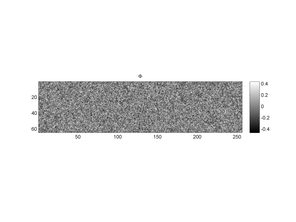
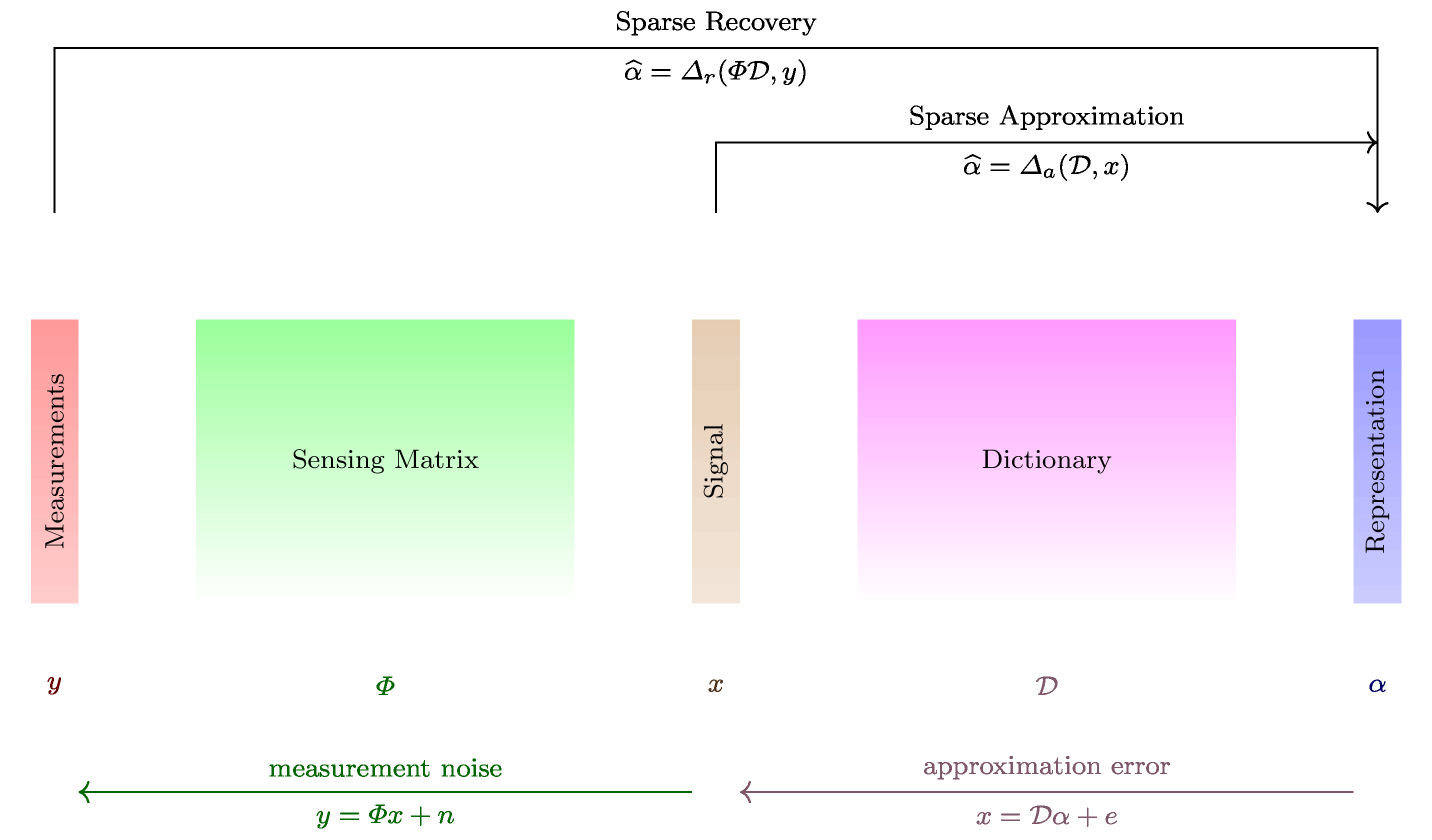
Fig. 18.13 A Gaussian sensing matrix of shape \(64 \times 256\). The sensing matrix maps signals from the space \(\RR^{256}\) to the measurement space \(\RR^{64}\).#
18.7.2. The Sensing Matrix#
There are two ways to look at the sensing matrix. First view is in terms of its columns
where \(\phi_i \in \CC^M\) are the columns of sensing matrix. In this view we see that
i.e., \(\by\) belongs to the column span of \(\Phi\) and one representation of \(\by\) in \(\Phi\) is given by \(x\).
This view looks very similar to a dictionary and its atoms but there is a difference. In a dictionary, we require each atom to be unit norm. We don’t require columns of the sensing matrix \(\Phi\) to be unit norm.
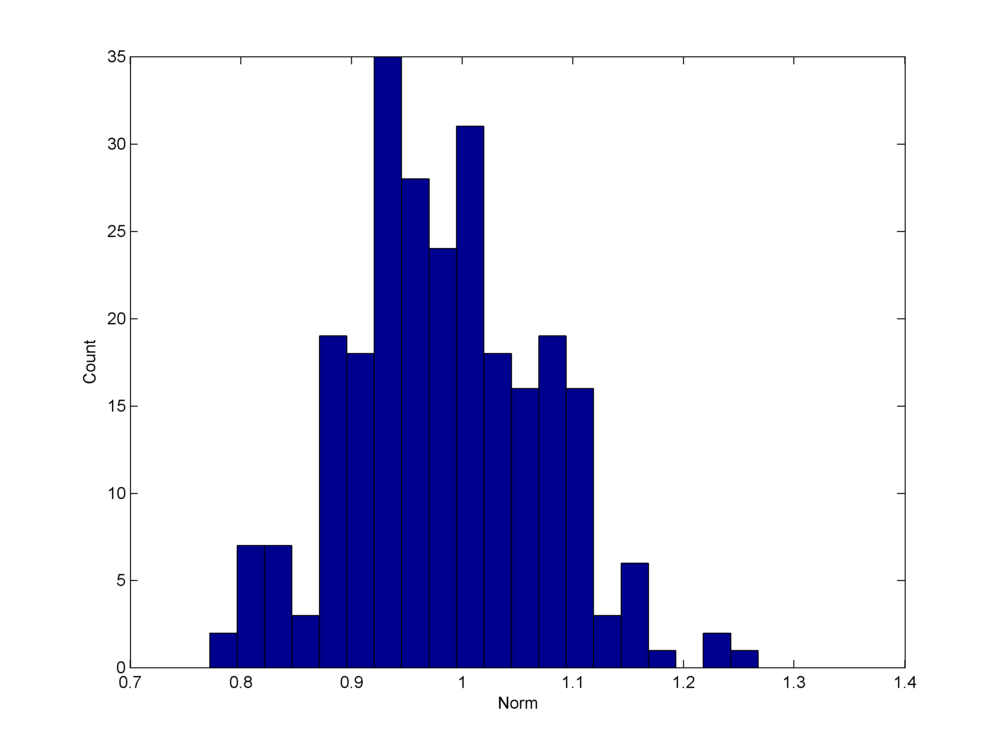
Fig. 18.14 A histogram of the norms of the columns of a Gaussian sensing matrix. Although the histogram is strongly concentrated around \(1\), yet there is significant variation in norm between \(0.75\) and \(1.3\). Compare this with the two ortho bases type dictionaries where by design all columns are unit norm.#
The second view of sensing matrix \(\Phi\) is in terms of its columns. We write
where \(\bf_i \in \CC^N\) are conjugate transposes of rows of \(\Phi\). This view gives us following expression:
In this view \(y_i\) is a measurement given by the inner product of \(\bx\) with \(\bf_i\) \(( \langle \bx , \bf_i \rangle = \bf_i^H \bx)\).
We will call \(\bf_i\) as a sensing vector. There are \(M\) such sensing vectors in \(\CC^N\) comprising \(\Phi\) corresponding to \(M\) measurements in the measurement space \(\CC^M\).
Definition 18.25 (Embedding of a signal)
Given a signal \(\bx \in \RR^N\), a vector \(\by = \Phi \bx \in \RR^M\) is called an embedding of \(\bx\) in the measurement space \(\RR^M\).
Definition 18.26 (Explanation of a measurement)
A signal \(\bx \in \RR^N\) is called an explanation of a measurement \(\by \in \RR^M\) w.r.t. sensing matrix \(\Phi\) if \(\by = \Phi \bx\).
Definition 18.27 (Measurement noise)
In real life, the measurement is not error free. It is affected by the presence of noise during measurement. This is modeled by the following equation:
where \(\be \in \RR^M\) is the measurement noise.
Example 18.27 (Compressive measurements of a synthetic sparse signal )
In this example we show:
A synthetic sparse signal
Its measurements using a Gaussian sensing matrix
Addition of noise during the measurement process.
Fig. 18.15 A \(4\)-sparse signal of length \(256\). The signal is assumed to be sparse in itself. Thus, we don’t require an orthonormal basis or a dictionary in which the signal has a sparse representation. We have \(N=256\) and \(K=4\).#
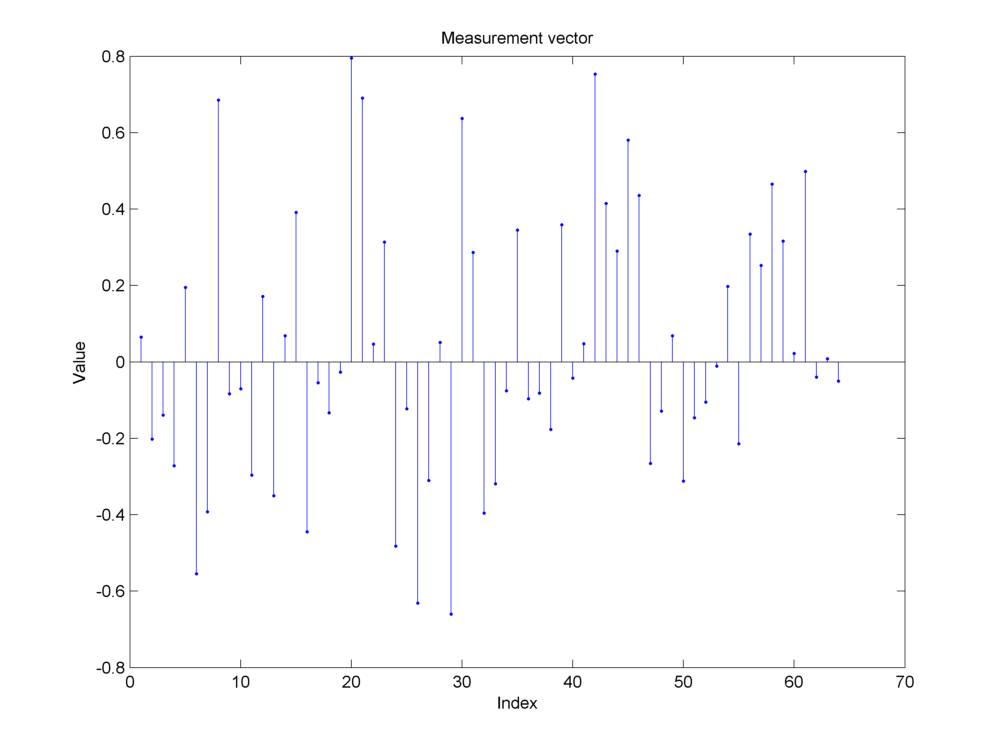
Fig. 18.16 Measurements made by a Gaussian sensing matrix \(\by = \Phi \bx\). The measurements are random. The original sparse structure is not clear by visual inspection.#
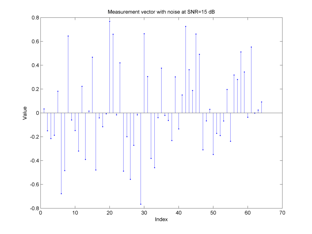
Fig. 18.17 Addition of measurement noise at an SNR of \(15\)dB.#
In Example 18.30, we show the reconstruction of the sparse signal from its measurements.
In the following we present examples of real life problems which can be modeled as compressive sensing problems.
18.7.3. Error Correction in Linear Codes#
The classical error correction problem was discussed in one of the seminal founding papers on compressive sensing [19].
Example 18.28 (Error correction in linear codes as a compressive sensing problem)
Let \(\bf \in \RR^N\) be a “plaintext” message being sent over a communication channel.
In order to make the message robust against errors in communication channel, we encode the error with an error correcting code.
We consider \(\bA \in \RR^{D \times N}\) with \(D > N\) as a linear code. \(\bA\) is essentially a collection of code words given by
where \(\ba_i \in \RR^D\) are the code words.
We construct the “ciphertext”
where \(\bx \in \RR^D\) is sent over the communication channel. Clearly \(\bx\) is a redundant representation of \(\bf\) which is expected to be robust against small errors during transmission.
\(\bA\) is assumed to be full column rank. Thus \(\bA^T \bA\) is invertible and we can easily see that
where
is the left pseudo inverse of \(\bA\).
The communication channel is going to add some error. What we actually receive is
where \(\be \in \RR^D\) is the error being introduced by the channel.
The least squares solution by minimizing the error \(\ell_2\) norm is given by
Since \(\bA^{\dag} \be\) is usually non-zero (we cannot assume that \(\bA^{\dag}\) will annihilate \(\be\)), hence \(\bf'\) is not an exact replica of \(\bf\).
What is needed is an exact reconstruction of \(\bf\). To achieve this, a common assumption in literature is that error vector \(\be\) is in fact sparse. i.e.
To reconstruct \(\bf\) it is sufficient to reconstruct \(\be\) since once \(\be\) is known we can get
and from there \(\bf\) can be faithfully reconstructed.
The question is: for a given sparsity level \(K\) for the error vector \(\be\) can one reconstruct \(\be\) via practical algorithms? By practical we mean algorithms which are of polynomial time w.r.t. the length of “ciphertext” (\(D\)).
The approach in [19] is as follows. We construct a matrix \(\bF \in \RR^{M \times D}\) which can annihilate \(\bA\); i.e.,
We then apply \(\bF\) to \(\by\) giving us
Therefore the decoding problem is reduced to that of reconstructing a sparse vector \(\be \in \RR^D\) from the measurements \(\bF \be \in \RR^M\) where we would like to have \(M \ll D\).
With this the problem of finding \(\be\) can be cast as problem of finding a sparse solution for the under-determined system given by
This now becomes the compressive sensing problem. The natural questions are
How many measurements \(M\) are necessary (in \(\bF\)) to be able to recover \(\be\) exactly?
How should \(\bF\) be constructed?
How do we recover \(\be\) from \(\tilde{\by}\)?
These problems are addressed in following chapters as we discuss sensing matrices and signal recovery algorithms.
18.7.4. Piecewise Cubic Polynomial Signal#
Example 18.29 (Piecewise cubic polynomial signal)
This example was discussed in [18]. Our signal of interest is a piecewise cubic polynomial signal as shown below.
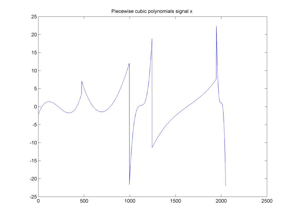
Fig. 18.18 A piecewise cubic polynomials signal#
It has a compressible representation in a wavelet basis.
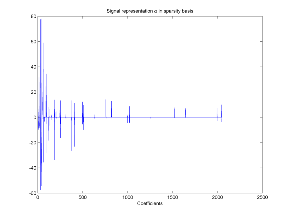
Fig. 18.19 Compressible representation of signal in wavelet basis#
The representation is described by the equation.
The chosen basis is a Daubechies wavelet basis \(\Psi\).
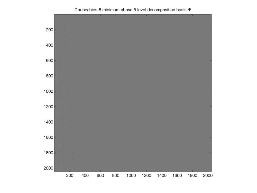
Fig. 18.20 Daubechies-8 wavelet basis#
In this example \(N = 2048\). We have \(\bx \in \RR^N\). \(\Psi\) is a complete dictionary of size \(N \times N\). Thus we have \(D = N\) and \(\alpha \in \RR^N\).
We can sort the wavelet coefficients by magnitude and plot them in descending order to visualize how sparse the representation is.
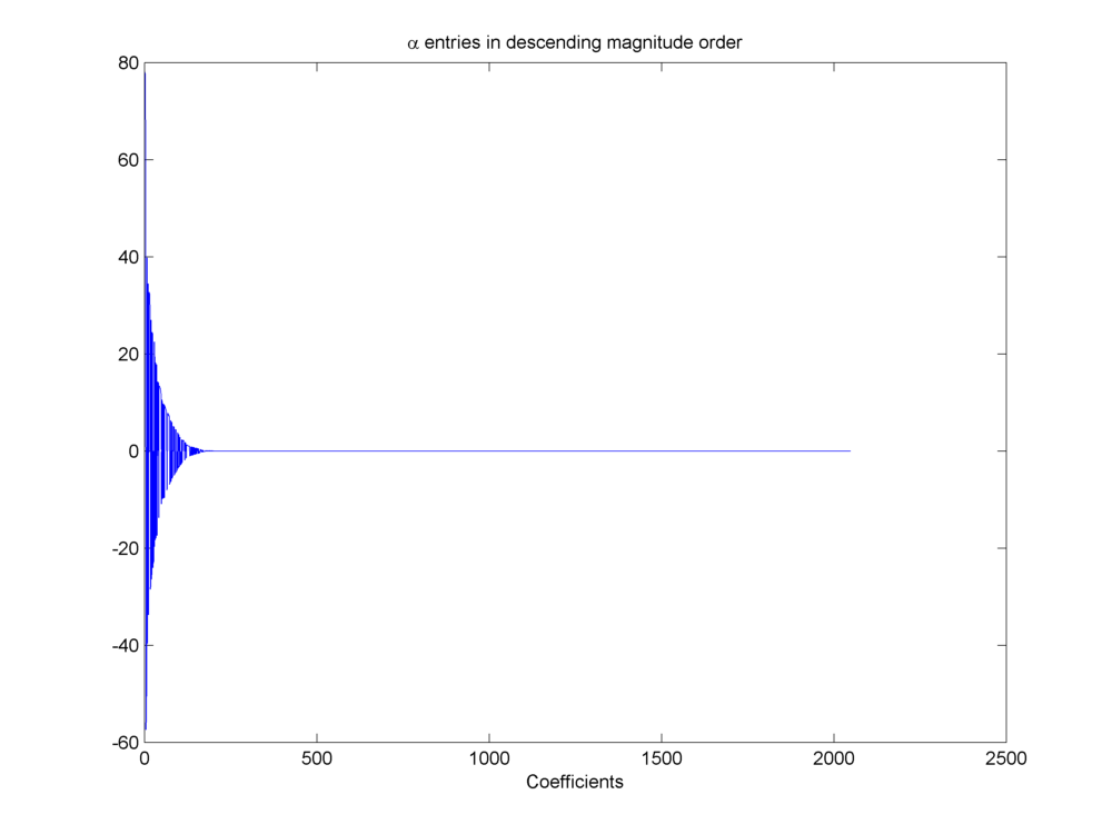
Fig. 18.21 Wavelet coefficients sorted by magnitude#
Before making compressive measurements, we need to decide how many compressive measurements will be sufficient?
Closely examining the coefficients in \(\alpha\) we can note that \(\max(\alpha_i) = 78.0546\). Further if we put different thresholds over magnitudes of entries in \(\alpha\) we can find the number of coefficients higher than different thresholds as listed below.
Entries in wavelet representation of piecewise cubic polynomial signal higher than a threshold
Threshold |
Entries higher than threshold |
|---|---|
1 |
129 |
1E-1 |
173 |
1E-2 |
186 |
1E-4 |
197 |
1E-8 |
199 |
1E-12 |
200 |
A choice of \(M = 600\) looks quite reasonable given the decay of entries in \(\alpha\). Later we shall provide theoretical bounds for choice of \(M\).
A Gaussian random sensing matrix \(\Phi\) is used to generate the compressed measurements.
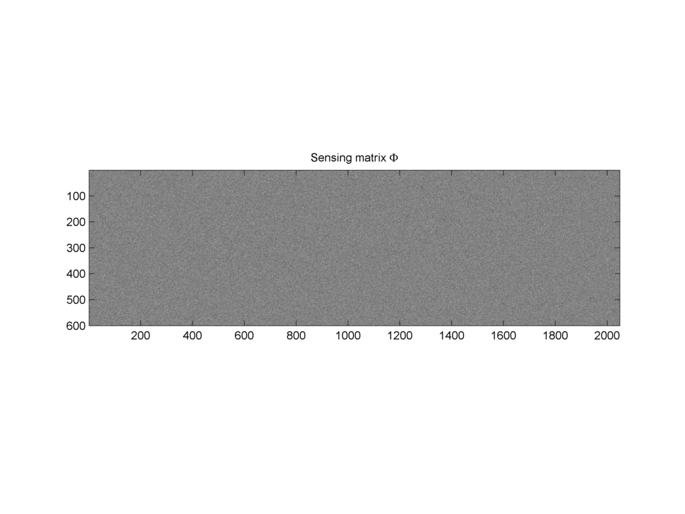
Fig. 18.22 Gaussian sensing matrix \(\Phi\)#
The measurement process is described by the equation
with \(\bx \in \RR^N\), \(\Phi \in \RR^{M \times N}\), and measurement vector \(\by \in \RR^M\). For this example we chose the measurement noise to be \(\be = \bzero\).
The compressed measurements are shown below.
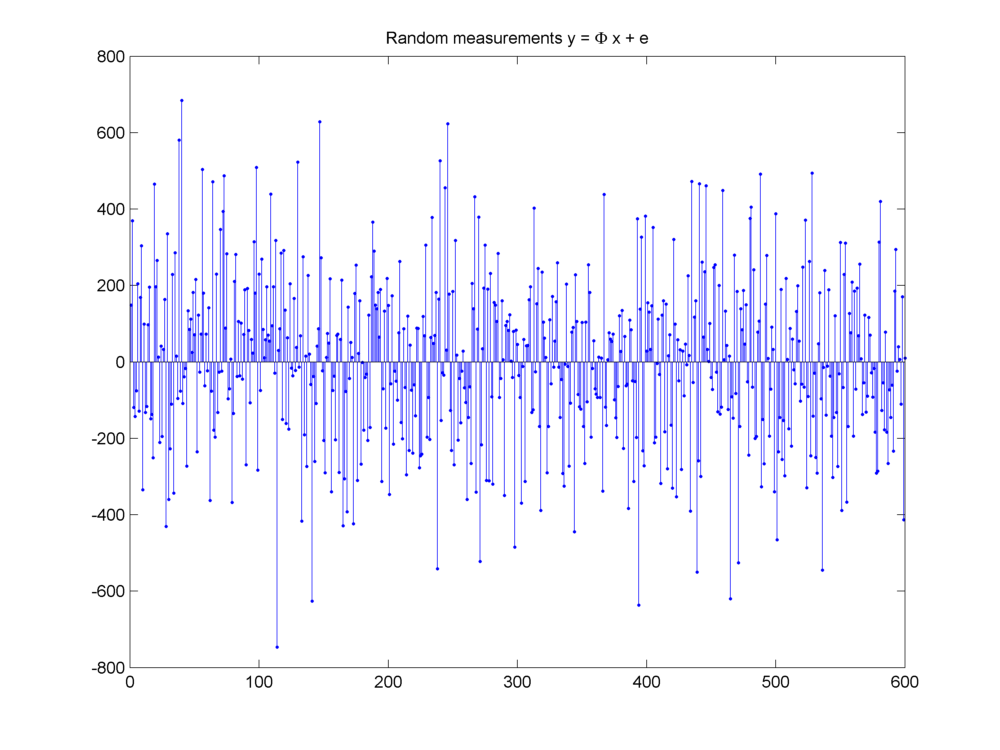
Fig. 18.23 Measurement vector \(\by = \Phi \bx + \be\)#
Finally the product of \(\Phi\) and \(\Psi\) given by \(\Phi \Psi\) will be used for actual recovery of sparse representation \(\alpha\) from the measurements \(\by\).
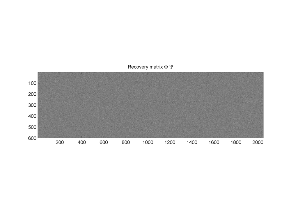
Fig. 18.24 Recovery matrix \(\Phi \Psi\)#
The sparse signal recovery problem is denoted as
where \(\widehat{\alpha}\) is a \(K\)-sparse approximation of \(\alpha\).
18.7.5. Number of Measurements#
A fundamental question of compressive sensing framework is: How many measurements are necessary to acquire \(K\)-sparse signals? By necessary we mean that \(\by\) carries enough information about \(\bx\) such that \(\bx\) can be recovered from \(\by\).
Clearly if \(M < K\) then recovery is not possible.
We further note that the sensing matrix \(\Phi\) should not map two different \(K\)-sparse signals to the same measurement vector. Thus we will need \(M \geq 2K\) and each collection of \(2K\) columns in \(\Phi\) must be non-singular.
If the \(K\)-column sub matrices of \(\Phi\) are badly conditioned, then it is possible that some sparse signals get mapped to very similar measurement vectors. Then it is numerically unstable to recover the signal. Moreover, if noise is present, stability further degrades.
In [20] Cand`es and Tao showed that the geometry of sparse signals should be preserved under the action of a sensing matrix. In particular the distance between two sparse signals shouldn’t change by much during sensing.
They quantified this idea in the form of a restricted isometric constant of a matrix \(\Phi\) as the smallest number \(\delta_K\) for which the following holds
We will study more about this property known as restricted isometry property (RIP) in Restricted Isometry Property. Here we just sketch the implications of RIP for compressive sensing.
When \(\delta_K < 1\) then the inequalities imply that every collection of \(K\) columns from \(\Phi\) is non-singular. Since we need every collection of \(2K\) columns to be non-singular, we actually need \(\delta_{2K} < 1\) which is the minimum requirement for recovery of \(K\) sparse signals.
Further if \(\delta_{2K} \ll 1\) then we note that sensing operator very nearly maintains the \(\ell_2\) distance between any two \(K\) sparse signals. As a consequence, it is possible to invert the sensing process stably.
It is now known that many randomly generated matrices have excellent RIP behavior. One can show that if \(\delta_{2K} \leq 0.1\), then with
measurements, one can recover \(\bx\) with high probability.
Some of the typical random matrices which have suitable RIP properties are
Gaussian sensing matrices
Partial Fourier matrices
Rademacher sensing matrices
18.7.6. Signal Recovery#
The second fundamental problem in compressive sensing is: Given the compressive measurements \(\by\) how do we recover the signal \(\bx\)? This problem is known as SPARSE-RECOVERY problem.
A simple formulation of the problem as: minimize \(\| \bx \|_0\) subject to \(\by = \Phi \bx\) is hopeless since it entails a combinatorial explosion of search space.
Over the years, people have developed a number of algorithms to tackle the sparse recovery problem.
The algorithms can be broadly classified into following categories
[Greedy pursuits] These algorithms attempt to build the approximation of the signal iteratively by making locally optimal choices at each step. Examples of such algorithms include OMP (orthogonal matching pursuit), stage-wise OMP, regularized OMP, CoSaMP (compressive sampling pursuit) and IHT (iterative hard thresholding).
[Convex relaxation] These techniques relax the \(\ell_0\) “norm” minimization problem into a suitable problem which is a convex optimization problem. This relaxation is valid for a large class of signals of interest. Once the problem has been formulated as a convex optimization problem, a number of solutions are available, e.g. interior point methods, projected gradient methods and iterative thresholding.
[Combinatorial algorithms] These methods are based on research in group testing and are specifically suited for situations where highly structured measurements of the signal are taken. This class includes algorithms like Fourier sampling, chaining pursuit, and HHS pursuit.
A major emphasis of these notes will be the study of these sparse recovery algorithms. We shall provide some basic results in this section. We shall work under the following framework in the remainder of this section.
Let \(\bx \in \RR^N\) be our signal of interest where \(N\) is the number of signal components or dimension of the signal space \(\RR^N\).
Let us make \(M\) linear measurements of the signal.
The measurements are given by
\[ \by = \Phi \bx. \]\(\by \in \RR^M\) is our measurement vector in the measurement space \(\RR^M\) and \(M\) is the dimension of our measurement space.
\(\Phi\) is an \(M\times N\) matrix known as the sensing matrix.
\(M \ll N\), hence \(\Phi\) achieves a dimensionality reduction over \(\bx\).
We assume that measurements are non-adaptive; i.e., the matrix \(\Phi\) is predefined and doesn’t depend on \(\bx\).
The recovery process is denoted by
\[ \bx' = \Delta \by = \Delta (\Phi \bx) \]where \(\Delta : \RR^M \to \RR^N\) is a (usually nonlinear) recovery algorithm.
We will look at three kinds of situations:
Signals are truly sparse. A signal has up to \(K (K \ll N)\) non-zero values only where \(K\) is known in advance. Measurement process is ideal and no noise is introduced during measurement. We will look for guarantees which can ensure exact recovery of signal from \(M (K < M \ll N)\) linear measurements.
Signals are not truly sparse but they have few \(K (K \ll N)\) values which dominate the signal. Thus if we approximate the signal by these \(K\) values, then approximation error is not noticeable. We again assume that there is no measurement noise being introduced. When we recover the signal, it will in general not be exact recovery. We expect the recovery error to be bounded (by approximation error). Also in special cases where the signal turns out to be \(K\)-sparse, we expect the recovery algorithm to recover the signal exactly. Such an algorithm with bounded recovery error will be called robust.
Signals are not sparse. Also there is measurement noise being introduced. We expect recovery algorithm to minimize error and thus perform stable recovery in the presence of measurement noise.
Example 18.30 (Reconstruction of the synthetic sparse signal from its noisy measurements)
Continuing from Example 18.27, we show the approximation reconstruction of the synthetic sparse signal using 3 different algorithms.
Basis pursuit (\(\ell_1\) minimization) algorithm
Matching pursuit algorithm
Orthogonal matching pursuit algorithm
The reconstructions are not exact due to the presence of measurement noise.
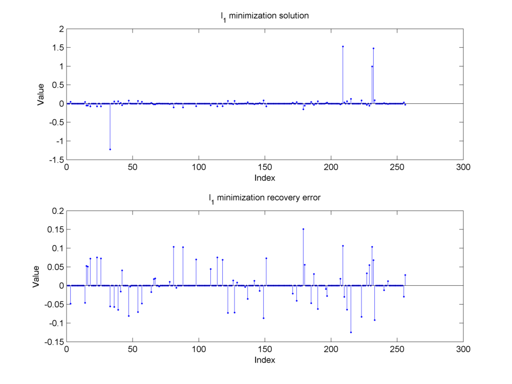
Fig. 18.25 Reconstruction of the sparse signal using \(\ell_1\) minimization (basis pursuit). If we compare with the original signal in Fig. 18.15, we can see that the algorithm has been able to recover the large nonzero entries pretty closely. However, there is still some amount of reconstruction error at other indices outside the support of the original signal due to the presence of measurement noise.#
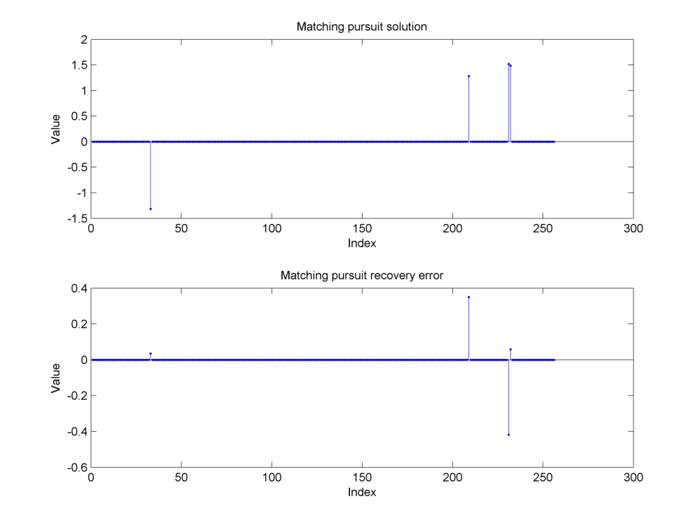
Fig. 18.26 Reconstruction of the sparse signal using matching pursuit. The support of the original signal has been identified correctly but matching pursuit hasn’t been able to get the magnitude of these components correctly. Some energy seems to have been transferred between the nearby second and third nonzero components. This is clear from the large magnitude in the recovery error at the second and third components. The presence of measurement noise affects simple algorithms like matching pursuit severely.#
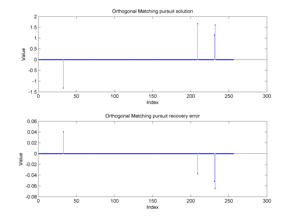
Fig. 18.27 Reconstruction of the sparse signal using orthogonal matching pursuit. The support has been identified correctly and the magnitude of the nonzero components in the reconstructed signal is close to the original signal. The reconstruction error is primarily due to the presence of measurement noise. It is roughly evenly distributed between all the nonzero entries since orthogonal matching pursuit computes a least squares solution over the selected indices in the support.#
18.7.7. Exact Recovery of Sparse Signals#
The null space of a matrix \(\Phi\) is denoted as
The set of \(K\)-sparse signals is defined as
Example 18.31 (K sparse signals)
Let \(N=10\).
\(\bx=(1,2, 1, -1, 2 , -3, 4, -2, 2, -2) \in \RR^{10}\) is not a sparse signal.
\(\bx=(0,0,0,0,1,0,0,-1,0,0)\in \RR^{10}\) is a 2-sparse signal. Its also a 4 sparse signal.
Lemma 18.2
If \(\ba\) and \(\bb\) are two \(K\) sparse signals then \(\ba - \bb\) is a \(2K\) sparse signal.
Proof. \((a - b)_i\) is non zero only if at least one of \(a_i\) and \(b_i\) is non-zero. Hence number of non-zero components of \(\ba - \bb\) cannot exceed \(2K\). Hence \(\ba - \bb\) is a \(2K\)-sparse signal.
Example 18.32 (Difference of K sparse signals)
Let N = 5.
Let \(\ba = (0,1,-1,0, 0)\) and \(\bb = (0,2,0,-1, 0)\). Then \(\ba - \bb = (0,-1,-1,1, 0) \) is a 3 sparse as well as 4 sparse signal.
Let \(\ba = (0,1,-1,0, 0)\) and \(\bb = (0,2,-1,0, 0)\). Then \(\ba - \bb = (0,-1,-2,0, 0) \) is a 2 sparse as well as 4 sparse signal.
Let \(\ba = (0,1,-1,0, 0)\) and \(\bb = (0,0,0,1, -1)\). Then \(\ba - \bb = (0,1,-1,-1, 1) \) is a 4 sparse signal.
Definition 18.28 (Unique embedding of a set)
We say that a sensing matrix \(\Phi\) uniquely embeds a set \(C \subseteq \RR^N\) if for any \(\ba, \bb \in C\), we have
Theorem 18.38 (Unique embeddings of \(K\) sparse vectors)
A sensing matrix \(\Phi\) uniquely embeds every \(\bx \in \Sigma_K\) if and only if \(\NullSpace(\Phi) \cap \Sigma_{2K} = \EmptySet\); i.e., \(\NullSpace(\Phi)\) contains no vectors in \(\Sigma_{2K}\).
Proof. We first show that the difference of sparse signals is not in the nullspace.
Let \(\ba\) and \(\bb\) be two \(K\) sparse signals.
Then \(\Phi \ba\) and \(\Phi \bb\) are corresponding measurements.
Now if \(\Phi\) provides unique embedding of all \(K\) sparse signals, then \(\Phi \ba \neq \Phi \bb\).
Thus \(\Phi (\ba - \bb) \neq \bzero\).
Thus \(\ba - \bb \notin \NullSpace(\Phi)\).
We show the converse by contradiction.
Let \(\bx \in \NullSpace(\Phi) \cap \Sigma_{2K}\).
Thus \(\Phi \bx = \bzero\) and \(\|\bx\|_0 \leq 2K\).
Then we can find \(\by, \bz \in \Sigma_K\) such that \(\bx = \bz - \by\).
Thus there exists \(\bm \in \RR^M\) such that \(\bm = \Phi \bz = \Phi \by\).
But then, \(\Phi\) doesn’t uniquely embed \(\by, \bz \in \Sigma_K\).
There are equivalent ways of characterizing this condition. In the following, we present a condition based on spark.
18.7.7.1. Spark#
We recall from Definition 18.17, that spark of a matrix \(\Phi\) is defined as the minimum number of columns which are linearly dependent.
Theorem 18.39 (Unique explanations and spark)
For any measurement \(\by \in \RR^M\), there exists at most one signal \(\bx \in \Sigma_K\) such that \(\by = \Phi \bx\) if and only if \(\spark(\Phi) > 2K\).
Proof. We need to show
If for every measurement, there is only one \(K\)-sparse explanation, then \(\spark(\Phi) > 2K\).
If \(\spark(\Phi) > 2K\) then for every measurement, there is only one \(K\)-sparse explanation.
Assume that for every \(\by \in \RR^M\) there exists at most one signal \(\bx \in \Sigma_K\) such that \(\by = \Phi \bx\).
Now assume that \(\spark(\Phi) \leq 2K\).
Thus there exists a set of at most \(2K\) columns which are linearly dependent.
Thus there exists \(\bv \in \Sigma_{2K}\) such that \( \Phi \bv = \bzero\).
Thus \(\bv \in \NullSpace (\Phi)\).
Thus \(\Sigma_{2K} \cap \NullSpace (\Phi) \neq \EmptySet\).
Hence \(\Phi\) doesn’t uniquely embed each signal \(\bx \in \Sigma_K\). A contradiction.
Hence \(\spark(\Phi) > 2K\).
Now suppose that \(\spark(\Phi) > 2K\).
Assume that for some \(y\) there exist two different \(K\)-sparse explanations \(\bx, \bx'\) such that \(\by = \Phi \bx =\Phi \bx'\).
Then \(\Phi (\bx - \bx') = \bzero\).
Thus \(\bx - \bx' \in \NullSpace (\Phi)\) and \(\bx - \bx' \in \Sigma_{2K}\).
Hence, there exists a set of at most \(2K\) columns in \(\Phi\) which is linearly dependent.
Thus \(\spark(\Phi) \leq 2K\). A contradiction.
Hence, for every \(\by \in \RR^M\), there exists at most one \(\bx \in \Sigma_K\).
Since \(\spark(\Phi) \in [2, M+1]\) and we require that \(\spark(\Phi) > 2K\) hence we require that \(M \geq 2K\).
18.7.8. Recovery of Approximately Sparse Signals#
Spark is a useful criteria for characterization of sensing matrices for truly sparse signals. But this doesn’t work well for approximately sparse signals. We need to have more restrictive criteria on \(\Phi\) for ensuring recovery of approximately sparse signals from compressed measurements.
In this context we will deal with two types of errors:
Approximation error
Let us approximate a signal \(\bx\) using only \(K\) coefficients.
Let us call the approximation as \(\widehat{\bx}\).
Thus \(\be_a = (\bx - \widehat{\bx})\) is approximation error.
Recovery error
Let \(\Phi\) be a sensing matrix.
Let \(\Delta\) be a recovery algorithm.
Then \(\bx'= \Delta(\Phi \bx)\) is the recovered signal vector.
The error \(\be_r = (\bx - \bx')\) is recovery error.
Ideally, the recovery error should not be too large compared to the approximation error.
In this following we will
Formalize the notion of null space property (NSP) of a matrix \(\Phi\).
Describe a measure for performance of an arbitrary recovery algorithm \(\Delta\).
Establish the connection between NSP and performance guarantee for recovery algorithms.
Suppose we approximate \(\bx\) by a \(K\)-sparse signal \(\widehat{\bx} \in \Sigma_K\), then the minimum error under \(\ell_p\) norm is given by
One specific \(\widehat{\bx} \in \Sigma_K\) for which this minimum is achieved is the best \(K\)-term approximation (Theorem 18.18).
In the following, we will need some additional notation.
Let \( I = \{1,2,\dots, N\}\) be the set of indices for signal \(\bx \in \RR^N\).
Let \(\Lambda \subset I\) be a subset of indices.
Let \(\Lambda^c = I \setminus \Lambda\).
\(\bx_{\Lambda}\) will denote a signal vector obtained by setting the entries of \(\bx\) indexed by \(\Lambda^c\) to zero.
Example 18.33
Let N = 4.
Then \(I = \{1,2,3,4\}\).
Let \(\Lambda = \{1,3\}\).
Then \(\Lambda^c = \{2, 4\}\).
Now let \(\bx = (-1,1,2,-4)\).
Then \(\bx_{\Lambda} = (-1, 0, 2, 0)\).
\(\Phi_{\Lambda}\) will denote a \(M\times N\) matrix obtained by setting the columns of \(\Phi\) indexed by \(\Lambda^c\) to zero.
Example 18.34
Let N = 4.
Then \(I = \{1,2,3,4\}\).
Let \(\Lambda = \{1,3\}\).
Then \(\Lambda^c = \{2, 4\}\).
Now let \(\bx = (-1,1,2,-4)\).
Then \(\bx_{\Lambda} = (-1, 0, 2, -4)\).
Now let
\[\begin{split} \Phi = \begin{pmatrix} 1 & 0 & -1 & 1\\ -1 & -2 & 2 & 3 \end{pmatrix}. \end{split}\]Then
\[\begin{split} \Phi_{\Lambda} = \begin{pmatrix} 1 & 0 & -1 & 0\\ -1 & 0 & 2 & 0 \end{pmatrix}. \end{split}\]
18.7.8.1. Null Space Property#
Definition 18.29 (Null space property)
A matrix \(\Phi\) satisfies the null space property (NSP) of order \(K\) if there exists a constant \(C > 0\) such that,
holds for every \(\bh \in \NullSpace (\Phi)\) and for every \(\Lambda\) such that \(|\Lambda| \leq K\).
Let \(\bh\) be \(K\) sparse. Thus choosing the indices on which \(\bh\) is non-zero, I can construct a \(\Lambda\) such that \(|\Lambda| \leq K\) and \(\bh_{{\Lambda}^c} = 0\). Thus \(\| \bh_{{\Lambda}^c}\|_1\) = 0. Hence above condition is not satisfied. Thus such a vector \(\bh\) should not belong to \(\NullSpace(\Phi)\) if \(\Phi\) satisfies NSP.
Essentially vectors in \(\NullSpace (\Phi)\) shouldn’t be concentrated in a small subset of indices.
If \(\Phi\) satisfies NSP then the only \(K\)-sparse vector in \(\NullSpace(\Phi)\) is \(\bh = \bzero\).
18.7.8.2. Measuring the Performance of a Recovery Algorithm#
Let \(\Delta : \RR^M \to \RR^N\) represent a recovery method to recover approximately sparse \(\bx\) from \(\by\).
\(\ell_2\) recovery error is given by
The \(\ell_1\) error for \(K\)-term approximation is given by \(\sigma_K(\bx)_1\).
We will be interested in guarantees of the form
Why, this recovery guarantee formulation?
Exact recovery of K-sparse signals. \(\sigma_K (\bx)_1 = 0\) if \(\bx \in \Sigma_K\).
Robust recovery of non-sparse signals
Recovery dependent on how well the signals are approximated by \(K\)-sparse vectors.
Such guarantees are known as instance optimal guarantees.
Also known as uniform guarantees.
Why the specific choice of norms?
Different choices of \(\ell_p\) norms lead to different guarantees.
\(\ell_2\) norm on the LHS is a typical least squares error.
\(\ell_2\) norm on the RHS will require prohibitively large number of measurements.
\(\ell_1\) norm on the RHS helps us keep the number of measurements less.
If an algorithm \(\Delta\) provides instance optimal guarantees as defined above, what kind of requirements does it place on the sensing matrix \(\Phi\)?
We show that NSP of order \(2K\) is a necessary condition for providing uniform guarantees.
18.7.8.3. NSP and Instance Optimal Guarantees#
Theorem 18.40 (NSP and instance optimal guarantees)
Let \(\Phi : \RR^N \to \RR^M\) denote a sensing matrix and \(\Delta : \RR^M \to \RR^N\) denote an arbitrary recovery algorithm. If the pair \((\Phi, \Delta)\) satisfies instance optimal guarantee (18.39), then \(\Phi\) satisfies NSP of the order \(2K\).
Proof. We are given that
\((\Phi, \Delta)\) form an encoder-decoder pair.
Together, they satisfy instance optimal guarantee (18.39).
Thus they are able to recover all sparse signals exactly.
For non-sparse signals, they are able to recover their \(K\)-sparse approximation with bounded recovery error.
We need to show that if \(\bh \in \NullSpace(\Phi)\), then \(\bh\) satisfies
where \(\Lambda\) corresponds to \(2K\) largest magnitude entries in \(\bh\). Note that we have used \(2K\) in this expression, since we need to show that \(\Phi\) satisfies NSP of order \(2K\).
Let \(\bh \in \NullSpace(\Phi)\).
Let \(\Lambda\) be the indices corresponding to the \(2K\) largest entries of \(\bh\).
Then
\[ \bh = \bh_{\Lambda} + \bh_{\Lambda^c}. \]Split \(\Lambda\) into \(\Lambda_0\) and \(\Lambda_1\) such that \(|\Lambda_0| = |\Lambda_1| = K\).
We have
\[ \bh_{\Lambda} = \bh_{\Lambda_0} + \bh_{\Lambda_1}. \]Let
\[ \bx = \bh_{\Lambda_0} + \bh_{\Lambda^c}. \]Let
\[ \bx' = - \bh_{\Lambda_1}. \]Then
\[ \bh = \bx - \bx'. \]By assumption \(\bh \in \NullSpace(\Phi)\).
Thus
\[ \Phi \bh = \Phi(\bx - \bx') = \bzero \implies \Phi \bx = \Phi \bx'. \]But since \(\bx' \in \Sigma_K\) (recall that \(\Lambda_1\) indexes only \(K\) entries) and \(\Delta\) is able to recover all \(K\)-sparse signals exactly, hence
\[ \bx' = \Delta (\Phi \bx'). \]Thus
\[ \Delta (\Phi \bx) = \Delta (\Phi \bx') = \bx'; \]i.e., the recovery algorithm \(\Delta\) recovers \(\bx'\) for the signal \(\bx\).
Certainly \(\bx\) is not \(K\)-sparse since \(\Delta\) recovers every \(K\)-sparse signal uniquely.
Hence \(\Lambda^c\) must be nonempty.
Finally we also have
\[ \| \bh_{\Lambda} \|_2 \leq \| \bh \|_2 = \| \bx - \bx'\|_2 = \| \bx - \Delta (\Phi \bx)\| _2 \]since \(\bh\) contains some additional non-zero entries.
But as per instance optimal recovery guarantee (18.39) for \((\Phi, \Delta)\) pair, we have
\[ \| \Delta (\Phi \bx) - \bx \|_2 \leq C \frac{\sigma_K (\bx)_1}{\sqrt{K}}. \]Thus
\[ \| \bh_{\Lambda} \|_2 \leq C \frac{\sigma_K (\bx)_1}{\sqrt{K}}. \]But
\[ \sigma_K (\bx)_1 = \min_{\widehat{x} \in \Sigma_K} \|\bx - \widehat{\bx}\|_1. \]Recall that \(\bx =\bh_{\Lambda_0} + \bh_{\Lambda^c}\) where \(\Lambda_0\) indexes \(K\) entries of \(\bh\) which are (magnitude wise) larger than all entries indexed by \(\Lambda^c\).
Hence the best \(\ell_1\)-norm \(K\) term approximation of \(\bx\) is given by \(\bh_{\Lambda_0}\).
Hence
\[ \sigma_K (\bx)_1 = \| \bh_{\Lambda^c} \|_1. \]Thus we finally have
\[ \| \bh_{\Lambda} \|_2 \leq C \frac{\| \bh_{\Lambda^c} \|_1}{\sqrt{K}} = \sqrt{2}C \frac{\| \bh_{\Lambda^c} \|_1}{\sqrt{2K}} \quad \Forall \bh \in \NullSpace(\Phi). \]Thus \(\Phi\) satisfies the NSP of order \(2K\).
It turns out that NSP of order \(2K\) is also sufficient to establish a guarantee of the form above for a practical recovery algorithm.
18.7.9. Recovery in Presence of Measurement Noise#
Measurement vector in the presence of noise is given by
where \(\be\) is the measurement noise or error. \(\| \be \|_2\) is the \(\ell_2\) size of measurement error.
Recovery error as usual is given by
Stability of a recovery algorithm is characterized by comparing variation of recovery error w.r.t. measurement error.
NSP is both necessary and sufficient for establishing guarantees of the form:
These guarantees do not account for presence of noise during measurement.
We need stronger conditions for handling noise. The restricted isometry property for sensing matrices comes to our rescue.
18.7.9.1. Restricted Isometry Property#
We recall that a matrix \(\Phi\) satisfies the restricted isometry property (RIP) of order \(K\) if there exists \(\delta_K \in (0,1)\) such that
holds for every \(\bx \in \Sigma_K = \{ \bx \ST \| \bx\|_0 \leq K \}\).
If a matrix satisfies RIP of order \(K\), then we can see that it approximately preserves the size of a \(K\)-sparse vector.
If a matrix satisfies RIP of order \(2K\), then we can see that it approximately preserves the distance between any two \(K\)-sparse vectors since difference vectors would be \(2K\) sparse (see Theorem 18.49) .
We say that the matrix is nearly orthonormal for sparse vectors.
If a matrix satisfies RIP of order \(K\) with a constant \(\delta_K\), it automatically satisfies RIP of any order \(K' < K\) with a constant \(\delta_{K'} \leq \delta_{K}\).
18.7.9.2. Stability#
Informally a recovery algorithm is stable if recovery error is small in the presence of small measurement noise.
Is RIP necessary and sufficient for sparse signal recovery from noisy measurements? Let us look at the necessary part.
We will define a notion of stability of the recovery algorithm.
Definition 18.30 (\(C\) stable encoder-decoder pair)
Let \(\Phi : \RR^N \to \RR^M\) be a sensing matrix and \(\Delta : \RR^M \to \RR^N\) be a recovery algorithm. We say that the pair \((\Phi, \Delta)\) is \(C\)-stable if for any \(\bx \in \Sigma_K\) and any \(\be \in \RR^M\) we have that
Error is added to the measurements.
LHS is \(\ell_2\) norm of recovery error.
RHS consists of scaling of the \(\ell_2\) norm of measurement error.
The definition says that recovery error is bounded by a multiple of the measurement error.
Thus adding a small amount of measurement noise shouldn’t be causing arbitrarily large recovery error.
It turns out that \(C\)-stability requires \(\Phi\) to satisfy RIP.
Theorem 18.41 (Necessity of RIP for \(C\)-stability)
If a pair \((\Phi, \Delta)\) is \(C\)-stable then
for all \(\bx \in \Sigma_{2K}\).
Proof. Remember that any \(\bx \in \Sigma_{2K}\) can be written in the form of \(\bx = \by - \bz\) where \(\by, \bz \in \Sigma_K\).
Let \(\bx \in \Sigma_{2K}\).
Split it in the form of \(\bx = \by -\bz\) with \(\by, \bz \in \Sigma_{K}\).
Define
\[ \be_y = \frac{\Phi (\bz - \by)}{2} \quad \text{and} \quad \be_z = \frac{\Phi (\by - \bz)}{2}. \]Thus
\[ \be_y - \be_z = \Phi (\bz - \by) \implies \Phi \by + \be_y = \Phi \bz + \be_z. \]We have
\[ \Phi \by + \be_y = \Phi \bz + \be_z = \frac{\Phi (\by + \bz)}{2}. \]Also we have
\[ \| \be_y \|_2 = \| \be_z \|_2 = \frac{\| \Phi (\by - \bz) \|_2}{2} = \frac{\| \Phi \bx \|_2}{2}. \]Let
\[ \by' = \Delta (\Phi \by + \be_y) = \Delta (\Phi \bz + \be_z). \]Since \((\Phi, \Delta)\) is \(C\)-stable, hence we have
\[ \| \by'- \by\|_2 \leq C \| \be_y\|_2. \]Also
\[ \| \by'- \bz\|_2 \leq C \| \be_z\|_2. \]Using the triangle inequality
\[\begin{split} \| \bx \|_2 &= \| \by - \bz\|_2 = \| \by - \by' + \by' - \bz \|_2\\ &\leq \| \by - \by' \|_2 + \| \by' - \bz\|_2\\ &\leq C \| \be_y \|_2 + C \| \be_z \|_2 = C (\| \be_y \|_2 + \| \be_z \|_2) = C \| \Phi \bx \|_2. \end{split}\]Thus we have for every \(\bx \in \Sigma_{2K}\)
\[ \frac{1}{C}\| \bx \|_2 \leq \| \Phi \bx \|_2. \]
This theorem gives us the lower bound for RIP property of order \(2K\) in (18.38) with \(\delta_{2K} = 1 - \frac{1}{C^2}\) as a necessary condition for \(C\)-stable recovery algorithms.
Note that smaller the constant \(C\), lower is the bound on recovery error (w.r.t. measurement error). But as \(C \to 1\), \( \delta_{2K} \to 0\), thus reducing the impact of measurement noise requires sensing matrix \(\Phi\) to be designed with tighter RIP constraints.
This result doesn’t require an upper bound on the RIP property in (18.38).
It turns out that If \(\Phi\) satisfies RIP, then this is also sufficient for a variety of algorithms to be able to successfully recover a sparse signal from noisy measurements. We will discuss this later.
18.7.9.3. Measurement Bounds#
As stated in previous section, for a \((\Phi, \Delta)\) pair to be \(C\)-stable we require that \(\Phi\) satisfies RIP of order \(2K\) with a constant \(\delta_{2K}\). Let us ignore \(\delta_{2K}\) for the time being and look at relationship between \(M\), \(N\) and \(K\). We have a sensing matrix \(\Phi\) of size \(M\times N\) and expect it to provide RIP of order \(2K\). How many measurements \(M\) are necessary? We will assume that \(K < N / 2\). This assumption is valid for approximately sparse signals.
Before we start figuring out the bounds, let us develop a special subset of \(\Sigma_K\) sets. Consider the set
When we say \( \| \bx\|_0 = K\), we mean that exactly \(K\) terms in each member of \(U\) can be non-zero (i.e. \(-1\) or \(+1\)).
Hence \(U\) is a set of signal vectors \(\bx\) of length \(N\) where each sample takes values from \(\{0, +1, -1\}\) and number of allowed non-zero samples is fixed at \(K\). An example below explains it further.
Example 18.35 (\(U\) for \(N=6\) and \(K=2\))
Each vector in \(U\) will have 6 elements out of which \(2\) can be non zero. There are \(\binom{6}{2}\) ways of choosing the non-zero elements. Some of those sets are listed below as examples:
Revisiting
It is now obvious that
Since there are \(\binom{N}{K}\) ways of choosing \(K\) non-zero elements and each non zero element can take either of the two values \(+1\) or \(-1\), hence the cardinality of set \(U\) is given by:
By definition
Further Let \(\bx, \by \in U\).
Then \(\bx - \by\) will have a maximum of \(2K\) non-zero elements.
The non-zero elements would have values in \(\{-2,-1,1,2\}\).
Thus \( \|\bx - \by \|_0 = R \leq 2K\).
Further \(\| \bx - \by \|_2^2 \geq R\).
Hence
We now state a result which will help us in getting to the bounds.
Lemma 18.3
Let \(K\) and \(N\) satisfying \(K < \frac{N}{2}\) be given. There exists a set \(X \subset \Sigma_K\) such that for any \(\bx \in X\) we have \(\|\bx \|_2 \leq \sqrt{K}\) and for any \(\bx, \by \in X\) with \(\bx \neq \by\),
and
Proof. We just need to find one set \(X\) which satisfies the requirements of this lemma. We have to construct a set \(X\) such that
\(\| \bx \|_2 \leq \sqrt{K} \Forall \bx \in X\).
\(\| \bx - \by \|_2 \geq \sqrt{\frac{K}{2}}\) for every \(bx, \by \in X\).
\(\ln | X | \geq \frac{K}{2} \ln \left( \frac{N}{K} \right)\) or equivalently \(|X| \geq \left( \frac{N}{K} \right)^{\frac{K}{2}}\).
First condition states that the set \(X\) lies in the intersection of \(\Sigma_K\) and the closed ball \(B[\bzero, \sqrt{K}]\). Second condition states that the points in \(X\) are sufficiently distant from each other. Third condition states that there are at least a certain number of points in \(X\).
We will construct \(X\) by picking vectors from \(U\). Thus \(X \subset U\).
Since \(\bx \in X \subset U\) hence \(\| \bx \|_2 = \sqrt{K} \leq \sqrt{K} \Forall \bx \in X\).
Consider any fixed \(\bx \in U\).
How many elements \(\by\) are there in \(U\) such that \(\|\bx - \by\|_2^2 < \frac{K}{2}\)?
Define
\[ U_x^2 = \left \{\by \in U \ST \|\bx - \by\|_2^2 < \frac{K}{2} \right \}. \]Clearly by requirements in the lemma, if \(\bx \in X\) then \(U_x^2 \cap X = \EmptySet\); i.e., no vector in \(U_x^2\) belongs to \(X\).
How many elements are there in \(U_x^2\)? Let us find an upper bound.
\(\Forall \bx, \by \in U\) we have \(\|\bx - \by\|_0 \leq \|\bx - \by\|_2^2\).
If \(\bx\) and \(\by\) differ in \(\frac{K}{2}\) or more places, then naturally \(\|\bx - \by\|_2^2 \geq \frac{K}{2}\).
Hence if \(\|\bx - \by\|_2^2 < \frac{K}{2}\) then \(\|\bx - \by\|_0 < \frac{K}{2}\) hence \(\|\bx - \by\|_0 \leq \frac{K}{2}\) for any \(\bx, \by \in U_x^2\).
So define
\[ U_x^0 = \left \{\by \in U \ST \|\bx - \by\|_0 \leq \frac{K}{2} \right \}. \]We have
\[ U_x^2 \subseteq U_x^0. \]Thus we have an upper bound given by
\[ | U_x^2 | \leq | U_x^0 |. \]Let us look at \(U_x^0\) carefully.
We can choose \(\frac{K}{2}\) indices where \(\bx\) and \(\by\) may differ in \(\binom{N}{\frac{K}{2}}\) ways.
At each of these \(\frac{K}{2}\) indices, \(y_i\) can take value as one of \((0, +1, -1)\).
Thus we have an upper bound
\[ | U_x^2 | \leq | U_x^0 | \leq \binom {N}{\frac{K}{2}} 3^{\frac{K}{2}}. \]We now describe an iterative process for building \(X\) from vectors in \(U\).
Say we have added \(j\) vectors to \(X\) namely \(x_1, x_2,\dots, x_j\).
Then
\[ (U^2_{x_1} \cup U^2_{x_2} \cup \dots \cup U^2_{x_j}) \cap X = \EmptySet. \]Number of vectors in \(U^2_{x_1} \cup U^2_{x_2} \cup \dots \cup U^2_{x_j}\) is bounded by \(j \binom {N}{ \frac{K}{2}} 3^{\frac{K}{2}}\).
Thus we have at least
\[ \binom{N}{K} 2^K - j \binom {N}{ \frac{K}{2}} 3^{\frac{K}{2}} \]vectors left in \(U\) to choose from for adding in \(X\).
We can keep adding vectors to \(X\) till there are no more suitable vectors left.
We can construct a set of size \(|X|\) provided
(18.40)#\[ |X| \binom {N}{ \frac{K}{2}} 3^{\frac{K}{2}} \leq \binom{N}{K} 2^K\]Now
\[ \frac{\binom{N}{K}}{\binom{N}{\frac{K}{2}}} = \frac {\left ( \frac{K}{2} \right ) ! \left (N - \frac{K}{2} \right ) ! } {K! (N-K)!} = \prod_{i=1}^{\frac{K}{2}} \frac{N - K + i}{ K/ 2 + i}. \]Note that \(\frac{N - K + i}{ K/ 2 + i}\) is a decreasing function of \(i\).
Its minimum value is achieved for \(i=\frac{K}{2}\) as \((\frac{N}{K} - \frac{1}{2})\).
So we have
\[\begin{split} &\frac{N - K + i}{ K/ 2 + i} \geq \frac{N}{K} - \frac{1}{2}\\ &\implies \prod_{i=1}^{\frac{K}{2}} \frac{N - K + i}{ K/ 2 + i} \geq \left ( \frac{N}{K} - \frac{1}{2} \right )^{\frac{K}{2}}\\ &\implies \frac{\binom{N}{K}}{\binom{N}{\frac{K}{2}}} \geq \left ( \frac{N}{K} - \frac{1}{2} \right )^{\frac{K}{2}} \end{split}\]Rephrasing the bound on \(|X\) in (18.40) we have
\[ |X| \left( \frac{3}{4} \right )^{\frac{K}{2}} \leq \frac{\binom{N}{K}}{\binom{N}{\frac{K}{2}}} \]Hence we can definitely construct a set \(X\) with the cardinality satisfying
\[ |X| \left( \frac{3}{4} \right ) ^{\frac{K}{2}} \leq \left ( \frac{N}{K} - \frac{1}{2} \right )^{\frac{K}{2}}. \]Now it is given that \( K < \frac{N}{2}\). So we have:
\[\begin{split} & K < \frac{N}{2}\\ &\implies \frac{N}{K} > 2\\ &\implies \frac{N}{4K} > \frac{1}{2}\\ &\implies \frac{N}{K} - \frac{N}{4K} < \frac{N}{K} - \frac{1}{2}\\ &\implies \frac{3N}{4K} < \frac{N}{K} - \frac{1}{2}\\ &\implies \left( \frac{3N}{4K} \right) ^ {\frac{K}{2}}< \left ( \frac{N}{K} - \frac{1}{2} \right )^{\frac{K}{2}}\\ \end{split}\]Thus we have
\[ \left( \frac{N}{K} \right) ^ {\frac{K}{2}} \left( \frac{3}{4} \right) ^ {\frac{K}{2}} < \frac{\binom{N}{K}}{\binom{N}{\frac{K}{2}}} \]Choose
\[ |X| = \left( \frac{N}{K} \right) ^ {\frac{K}{2}} \]Clearly this value of \(|X|\) satisfies (18.40).
Hence \(X\) can have at least these many elements.
Thus
\[\begin{split} &|X| \geq \left( \frac{N}{K} \right) ^ {\frac{K}{2}}\\ &\implies \ln |X| \geq \frac{K}{2} \ln \left( \frac{N}{K} \right) \end{split}\]which completes the proof.
We can now establish following bound on the required number of measurements to satisfy RIP.
At this moment, we won’t worry about exact value of \(\delta_{2K}\). We will just assume that \(\delta_{2K}\) is small in range \((0, \frac{1}{2}]\).
Theorem 18.42 (Minimum number of required measurements for RIP of order \(2K\))
Let \(\Phi\) be an \(M \times N\) matrix that satisfies RIP of order \(2K\) with constant \(\delta_{2K} \in (0, \frac{1}{2}]\). Then
where
Proof. Since \(\Phi\) satisfies RIP of order \(2K\) we have
Also
Consider the set \(X \subset U \subset \Sigma_K\) developed in Lemma 18.3. We have
Also
since \(\|\bx\|_2 \leq \sqrt{K} \Forall \bx \in X\). So we have a lower bound:
and an upper bound:
What do these bounds mean? Let us start with the lower bound.
\(\Phi \bx\) and \(\Phi \by\) are projections of \(\bx\) and \(\by\) in \(\RR^M\) (measurement space).
Construct \(\ell_2\) balls of radius \(\sqrt{\frac{K}{4}} / 2= \sqrt{\frac{K}{16}}\) in \(\RR^M\) around \(\Phi \bx\) and \(\Phi \by\).
Lower bound says that these balls are disjoint. Since \(\bx, \by\) are arbitrary, this applies to every \(\bx \in X\).
Upper bound tells us that all vectors \(\Phi \bx\) lie in a ball of radius \(\sqrt {\frac{3K}{2}}\) around origin in \(\RR^M\).
Thus the set of all balls lies within a larger ball of radius \(\sqrt {\frac{3K}{2}} + \sqrt{\frac{K}{16}}\) around origin in \(\RR^M\).
So we require that the volume of the larger ball MUST be greater than the sum of volumes of \(|X|\) individual balls.
Since volume of an \(\ell_2\) ball of radius \(r\) is proportional to \(r^M\), we have:
Again from Lemma 18.3 we have
Putting back we get
which establishes a lower bound on the number of measurements \(M\).
Example 18.36 (Lower bounds on \(M\) for RIP of order \(2K\))
\(N=1000, K=100 \implies M \geq 65\).
\(N=1000, K=200 \implies M \geq 91\).
\(N=1000, K=400 \implies M \geq 104\).
Some remarks are in order:
The theorem only establishes a necessary lower bound on \(M\). It doesn’t mean that if we choose an \(M\) larger than the lower bound then \(\Phi\) will have RIP of order \(2K\) with any constant \(\delta_{2K} \in (0, \frac{1}{2}]\).
The restriction \(\delta_{2K} \leq \frac{1}{2}\) is arbitrary and is made for convenience. In general, we can work with \(0 < \delta_{2K} \leq \delta_{\text{max}} < 1\) and develop the bounds accordingly.
This result fails to capture dependence of \(M\) on the RIP constant \(\delta_{2K}\) directly. Johnson-Lindenstrauss lemma helps us resolve this which concerns embeddings of finite sets of points in low-dimensional spaces.
We haven’t made significant efforts to optimize the constants. Still they are quite reasonable.
18.7.10. RIP and NSP#
RIP and NSP are connected. If a matrix \(\Phi\) satisfies RIP then it also satisfies NSP (under certain conditions).
Thus RIP is strictly stronger than NSP (under certain conditions).
We will need following lemma which applies to any arbitrary \(\bh \in \RR^N\). The lemma will be proved later.
Lemma 18.4
Suppose that \(\Phi\) satisfies RIP of order \(2K\). Let \(\bh \in \RR^N, \bh \neq \bzero\) be arbitrary. Let \(\Lambda_0\) be any subset of \(\{1,2,\dots, N\}\) such that \(|\Lambda_0| \leq K\).
Define \(\Lambda_1\) as the index set corresponding to the \(K\) entries of \(h_{\Lambda_0^c}\) with largest magnitude, and set \(\Lambda = \Lambda_0 \cup \Lambda_1\). Then
where
Let us understand this lemma a bit. If \(\bh \in \NullSpace (\Phi)\), then the lemma simplifies to
\(\Lambda_0\) maps to the initial few (\(K\) or less) elements we chose.
\(\Lambda_0^c\) maps to all other elements.
\(\Lambda_1\) maps to largest (in magnitude) \(K\) elements of \(\Lambda_0^c\).
\(h_{\Lambda}\) contains a maximum of \(2K\) non-zero elements.
\(\Phi\) satisfies RIP of order \(2K\).
Thus
\[ (1 - \delta_{2K}) \| \bh_{\Lambda} \|_2 \leq \| \Phi \bh_{\Lambda} \|_2 \leq (1 + \delta_{2K}) \| \bh_{\Lambda} \|_2. \]
We now state the connection between RIP and NSP.
Theorem 18.43
Suppose that \(\Phi\) satisfies RIP of order \(2K\) with \(\delta_{2K} < \sqrt{2} - 1\). Then \(\Phi\) satisfies the NSP of order \(2K\) with constant
Proof. We are given that
holds for all \(\bx \in \Sigma_{2K}\) where \(\delta_{2K} < \sqrt{2} - 1\). We have to show that:
holds \(\Forall \bh \in \NullSpace (\Phi)\) and \(\Forall \Lambda\) such that \(|\Lambda| \leq 2K\).
Let \(\bh \in \NullSpace(\Phi)\).
Then \( \Phi \bh = \bzero\).
Let \(\Lambda_m\) denote the \(2K\) largest entries of \(\bh\).
Then
\[ \| \bh_{\Lambda}\|_2 \leq \| \bh_{\Lambda_m}\|_2 \Forall \Lambda \ST |\Lambda| \leq 2K. \]Similarly
\[ \| \bh_{\Lambda^c}\|_1 \geq \| \bh_{\Lambda_m^c}\|_1 \Forall \Lambda \ST |\Lambda| \leq 2K. \]Thus if we show that \(\Phi\) satisfies NSP of order \(2K\) for \(\Lambda_m\); i.e.,
\[ \| \bh_{\Lambda_m}\|_2 \leq C \frac{\| \bh_{{\Lambda_m}^c}\|_1 }{\sqrt{K}} \]then we would have shown it for all \(\Lambda\) such that \(|\Lambda| \leq 2K\).
Hence let \(\Lambda = \Lambda_m\).
We can divide \(\Lambda\) into two components \(\Lambda_0\) and \(\Lambda_1\) of size \(K\) each.
Since \(\Lambda\) maps to the largest \(2K\) entries in \(\bh\), hence whatever entries we choose in \(\Lambda_0\), the largest \(K\) entries in \(\Lambda_0^c\) will be \(\Lambda_1\).
Hence as per Lemma 18.4 above, we have
\[ \| \bh_{\Lambda} \|_2 \leq \alpha \frac{\| \bh_{\Lambda_0^c}\|_1}{\sqrt{K}}. \]Also
\[ \Lambda = \Lambda_0 \cup \Lambda_1 \implies \Lambda_0 = \Lambda \setminus \Lambda_1 = \Lambda \cap \Lambda_1^c \implies \Lambda_0^c = \Lambda_1 \cup \Lambda^c. \]Thus we have
\[ \| \bh_{\Lambda_0^c} \|_1 = \| \bh_{\Lambda_1} \|_1 + \| \bh_{\Lambda^c} \|_1. \]We have to get rid of \(\Lambda_1\).
Since \(\bh_{\Lambda_1} \in \Sigma_K\), by applying Theorem 18.17 we get
\[ \| \bh_{\Lambda_1} \|_1 \leq \sqrt{K} \| \bh_{\Lambda_1} \|_2 \]Hence
\[ \| \bh_{\Lambda} \|_2 \leq \alpha \left ( \| \bh_{\Lambda_1} \|_2 + \frac{\| \bh_{\Lambda^c} \|_1}{\sqrt{K}} \right) \]But since \(\Lambda_1 \subset \Lambda\), hence \( \| \bh_{\Lambda_1} \|_2 \leq \| \bh_{\Lambda} \|_2\).
Hence
\[\begin{split} &\| \bh_{\Lambda} \|_2 \leq \alpha \left ( \| \bh_{\Lambda} \|_2 + \frac{\| \bh_{\Lambda^c} \|_1}{\sqrt{K}} \right)\\ \implies &(1 - \alpha) \| \bh_{\Lambda} \|_2 \leq \alpha \frac{\| \bh_{\Lambda^c} \|_1}{\sqrt{K}}\\ \implies &\| \bh_{\Lambda} \|_2 \leq \frac{\alpha}{1 - \alpha} \frac{\| \bh_{\Lambda^c} \|_1}{\sqrt{K}} \quad \text{ if } \alpha \leq 1. \end{split}\]Note that the inequality is also satisfied for \(\alpha = 1\) in which case, we don’t need to bring \(1-\alpha\) to denominator.
Now
\[\begin{split} &\alpha \leq 1\\ \implies &\frac{\sqrt{2} \delta_{2K}}{ 1 - \delta_{2K}} \leq 1 \\ \implies &\sqrt{2} \delta_{2K} \leq 1 - \delta_{2K}\\ \implies &(\sqrt{2} + 1) \delta_{2K} \leq 1\\ \implies &\delta_{2K} \leq \sqrt{2} - 1. \end{split}\]Putting
\[ C = \frac{\alpha}{1 - \alpha} = \frac {\sqrt{2} \delta_{2K}} {1 - (1 + \sqrt{2})\delta_{2K}} \]we see that \(\Phi\) satisfies NSP of order \(2K\) whenever \(\Phi\) satisfies RIP of order \(2K\) with \(\delta_{2K} \leq \sqrt{2} -1\).
Note that for \(\delta_{2K} = \sqrt{2} - 1\), \(C=\infty\).